Bayesian Regression in Julia (With an Ordered Categorical Predictor Variable)

Intro

In this post, we'll use a Bayesian regression model to estimate the incremental effects of education on income. We'll be working with the U.S. Census Bureau's 2020 American Community Survey public use microdata sample file for the U.S. state of Vermont.

The Data

The file that we'll be using can be downloaded from the Census Bureau's FTP site here. There are hundreds of variables available in the data set but we'll only be using a few throughout this post:

• PWGTP: Person's weight. This is needed to compute estimates that represent the entire population.
• SCHL: Educational attainment.
• ESR: Employment status.
• WAGP: Wages/salary income over the previous 12 months.

Data Prep

Let's now prepare our data so that it's ready for using:

using CSV
using DataFramesMeta
using StatsBase

function education(schl)
    if schl in 1:15
        return 1
    elseif schl in 16:19
        return 2
    elseif schl == 20
        return 3
    elseif schl == 21
        return 4
    elseif schl in 22:23
        return 5
    elseif schl == 24
        return 6
    else
        return missing
    end
end

vars = [:PWGTP, :SCHL, :ESR, :WAGP]

df = @chain CSV.read(
        raw"C:\Users\mthel\Data\Census Data\acs\csv_pvt\psam_p50.csv",
        DataFrame;
        select=vars
    ) begin
        @subset(@byrow :ESR == 1)
        @subset(@byrow !ismissing(:WAGP))
        @subset(@byrow !ismissing(:SCHL))
        @transform(:edu = education.(:SCHL))
        @transform(:inc = standardize(ZScoreTransform, Float64.(:WAGP)))
    end

N = 5_000
s = df[sample(axes(df, 1), pweights(df.PWGTP), N; replace = true), :]

The first thing we did was define a function that will take our SCHL variable and map it to one of 6 different levels. The data set includes 24 different levels of educational attainment but I've chosen to reduce that down to 6 to make this example simpler. Then, we read the file and filter the data to only include individuals that are employed. We do this by taking a subset of the data where the variable ESR is equal to 1 (employed and at work). We also check to make sure that the WAGP and SCHL variables are not missing, since those are the ones that we care about. Finally, we create two new columns in the dataset to hold our educational attainment variable edu and our standardized income variable inc. Standardizing the person's income makes it easier to define priors in our statistical model and it also makes the posterior sampling process more efficient.

In the next step, we defined a sample size of 5,000. We then took a weighted random sample from our data set, with replacement, so that we ended up with a smaller sample data set that is still representative of the population. This will make our sampling go a little faster and it will also allow us to see how sensitive our estimates are to changes in the sample.

Here's what our DataFrame looks like:

5000×6 DataFrame
  Row │ PWGTP  SCHL    WAGP    ESR     edu    inc       
      │ Int64  Int64?  Int64?  Int64?  Int64  Float64   
──────┼─────────────────────────────────────────────────
    1 │    78      18   28000       1      2  -0.32411
    2 │    22      16   32000       1      2  -0.242847
    3 │    11      22   30000       1      5  -0.283478
    4 │    30      19    1500       1      2  -0.862475
  ⋮   │   ⋮      ⋮       ⋮       ⋮       ⋮        ⋮
 4998 │    13      20   22000       1      3  -0.446004
 4999 │    25      21   30000       1      4  -0.283478
 5000 │    30      19   74000       1      2   0.610411
                                       4993 rows omitted

The Causal Model

Let's start with our causal model. In this case, our (over-simplified) causal model looks like this:

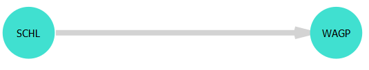
You can generate the above DAG with the following code:

using Dagitty

g = DAG(:SCHL => :WAGP)
drawdag(g, [0,1], [0, 0])

This simply states that we believe educational attainment directly affects a person's wage & salary income (and that nothing else does).

The Statistical Model

Now we can define our statistical model. Our predictor variable is an ordered categorical variable that looks like this:

1: Less than a high-school diploma
2: High-school diploma (or equivalent) and/or some college, but without a degree
3: Associate's degree
4: Bachelor's degree
5: Master's degree or another professional degree beyond a Bachelor's
6: Doctorate degree

We need our model to account for the possibility that the incremental effects might not be equal as you move from one level of education to another. In other words, the incremental effect on wages of obtaining an associate's degree may not be the same as the incremental effect of obtaining a doctorate degree. Let's go ahead and define the model and then we'll unpack it afterwards:

With this definition, we're stating that a person's standardized income is distributed normally. The mean $\mu$ contains our linear model, which consists of the sum of an intercept term $\alpha$ and the product of a coefficient $\beta$ and another term $\phi$ . Skipping down to our $\delta$ terms, they allow us to measure the effect of completing different levels of education and we are using a Dirichlet prior parameterized by a vector $A$ of length 5. We only need 5 values because we have 6 levels of educational attainment overall and the effect of the first level of educational attainment will be our base case (which will be accounted for in our intercept term). Moving back up to $\phi$ , we are taking the sum of all of the incremental effects that correspond to an individual's educational attainment. Note that when multiplying $\phi$ by our coefficient $\beta$ , we effectively capture the effect of the highest level of educational attainment, since all of our $\delta$ terms sum to 1. Finally, the vector $A$ consists of five 2s which represents a weak uniform prior for the incremental effects on wages of different levels of educational attainment.

Encoding Our Model With Turing.jl

We are now ready to build our model with Turing.jl. Here's the code:

using Turing

@model function education_model(wagp, schl)
    δ ~ Dirichlet(length(levels(schl)) - 1, 2)
    pushfirst!(δ, 0.0)
    α ~ Normal(0, 1.5)
    β ~ Normal(0, 1.5)
    Φ = sum.(map(i -> δ[1:i], schl))
    μ = @. α + β * Φ
    σ ~ Exponential(1)
    wagp ~ MvNormal(μ, σ)
end

Posterior Sampling

All that's left now is to run the model and obtain the samples from our posterior distribution:

m = education_model(s.inc, s.edu)
chain = sample(m, NUTS(), 1_000)

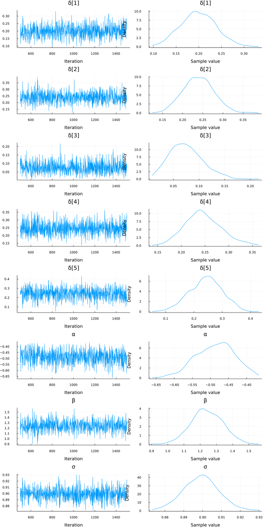
The summary statistics for our posterior look like this:

Summary Statistics
  parameters      mean       std   naive_se      mcse         ess      rhat   ess_per_sec 
      Symbol   Float64   Float64    Float64   Float64     Float64   Float64       Float64 

        δ[1]    0.1987    0.0390     0.0012    0.0014    790.7768    1.0003        1.8307
        δ[2]    0.2393    0.0384     0.0012    0.0013    825.1631    0.9990        1.9103
        δ[3]    0.0746    0.0323     0.0010    0.0012    987.2237    0.9998        2.2855
        δ[4]    0.2456    0.0384     0.0012    0.0012   1084.7209    0.9995        2.5112
        δ[5]    0.2418    0.0576     0.0018    0.0021    827.2804    0.9996        1.9152
           α   -0.4864    0.0535     0.0017    0.0020    775.4634    1.0007        1.7952
           β    1.2420    0.0993     0.0031    0.0039    747.3424    0.9991        1.7301
           σ    0.8992    0.0095     0.0003    0.0003    995.5158    1.0012        2.3046

Visualizing The Results

To visualize our posterior estimates:

using StatsPlots

plot(chain)

We can also create a nice visual of the incremental effects like this:

chaindf = DataFrame(chain)
μ = hcat(
    chaindf.α,
    [row.α + row.β * sum([row[eval("δ[$i]")] for i in 1:x]) for row in eachrow(chaindf), x in 1:5]
)
μ_mean = [mean(c) for c in eachcol(μ)]
μ_CI90 = hcat([percentile(c, [5,95]) for c in eachcol(μ)]...)'

plot(
    0:5,
    [μ_mean μ_mean],
    fillrange=μ_CI90,
    legend=false,
    color=:grey,
    alpha=0.5,
    linewidth=0
)

plot!(
    0:5,
    μ_mean,
    legend=false,
    xlabel="Educational Attainment",
    ylabel="Standardized Annual Income",
    marker=:o,
    title="Education Effect on Income",
    color=:purple
)

xticks!(0:5, ["No HS", "HS/Some College", "Associate's", "Bachelor's", "Master's", "Doctorate"])

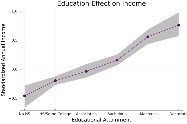
This shows us the mean standardized annual income that we expect at each level of educational attainment, as well as a 90% credible interval around that mean.

Finally, we can simulate some data from our posterior and add a 90% interval showing where our model expects the majority of incomes to be, given different levels of education:

sims = hcat(
    [rand(Normal(row.α, row.σ)) for row in eachrow(chaindf)],
    [rand(Normal(row.α + row.β * sum([row[eval("δ[$i]")] for i in 1:x]), row.σ)) for row in eachrow(chaindf), x in 1:5]
)

sims_CI90 = hcat([percentile(c, [5,95]) for c in eachcol(sims)]...)'

plot!(
    0:5,
    [μ_mean μ_mean],
    fillrange=sims_CI90,
    legend=false,
    color=:lightgrey,
    alpha=0.5,
    linewidth=0
)

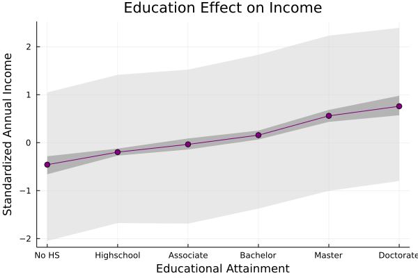
We can see that this produces a much wider range of possible values, which tells us that there are probably additional variables that determine an individual's income.

Final Thoughts

Thanks for reading. If you enjoyed this post, let me know. If you didn't enjoy it, let me know why. If you find mistakes (I'd be surprised if there wasn't at least one or two 😊), please point those out so that I can fix them!