Replacing legacy code with Julia

Introduction

At some point, students of the finite element method need to come to grips with sparse matrices. The finite element method is really viable only if it results in sufficiently sparse matrices. Firstly due to the reduction of the memory needed to store the matrix to the point where the data can be accommodated by the current hardware limits, and secondly because of the attendant gains in performance as the zero entries need not be processed.

Classical finite element approaches lead to matrices that are sparse, symmetric, and positive definite. One of the established techniques to deal with a sparse matrix is to allocate storage for the matrix entries below the so called envelope (sometimes referred to as skyline). Only one triangle of the matrix needs to be stored (either the lower or the upper). Here we assume that in each column we need to store only the entries below the top nonzero in that column and the diagonal.

Due to the expected properties of the matrices as outlined above, either a Cholesky or an LDL^T factorization of such matrices can be employed to solve a system of linear algebraic equations. Below we discuss the latter technique.

Gauss elimination

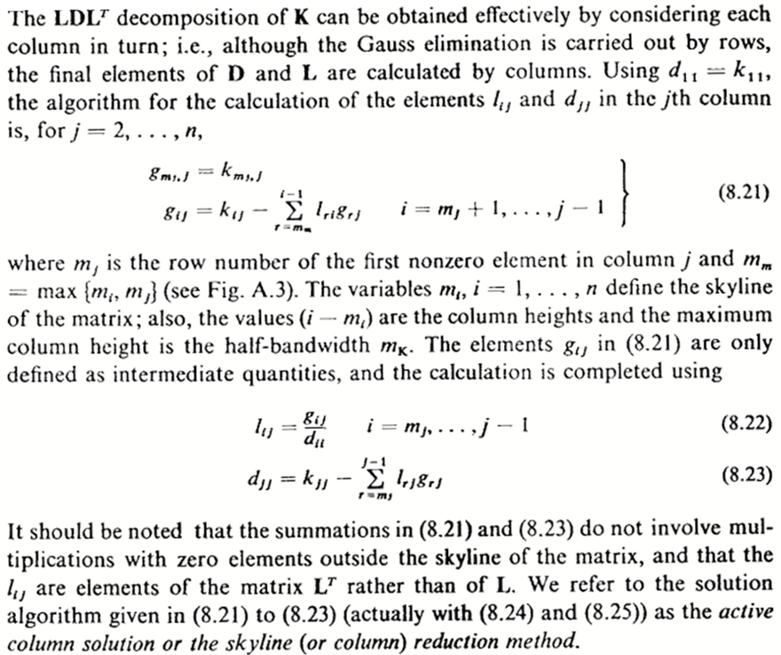
The textbook by Bathe¹ describes a sophisticated version of the Gauss elimination which operates on the upper triangle of the matrix, producing the entries of the L^T factor and the entries of the diagonal D. Figure 1 below is the complete description of the algorithm.

Figure 1: Active-column LDL^T factorization.

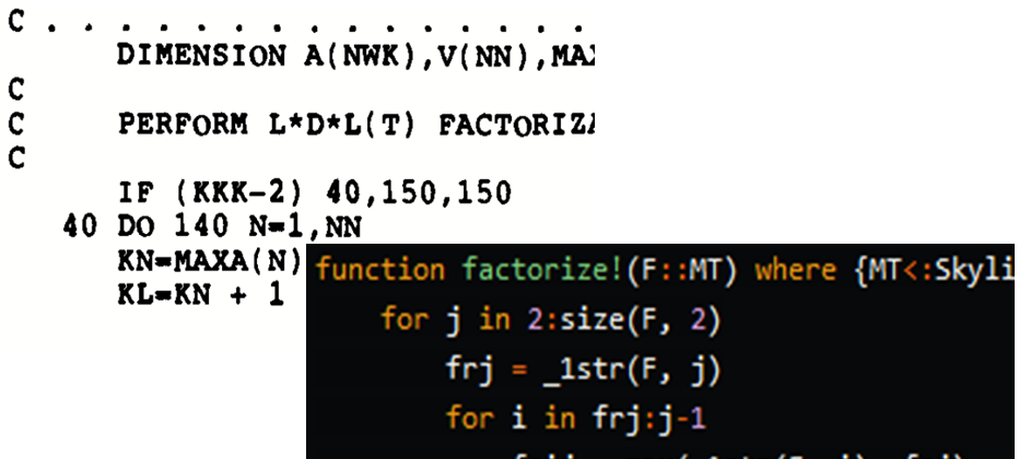
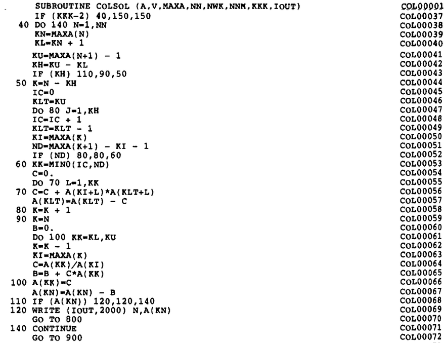
For a long time, the textbook by Bathe¹ served as a reference of the implementation (page 448). Figure 2 shows the Fortran code of the envelope-matrix factorization (originally in Fortran IV, later modified to Fortran 77) from this book.

Figure 2: Fortran implementation of the active-column LDL^T factorization.

Clearly, there is a wide chasm between the description of the algorithm and the code that implements it. Of course, the archaic form of the Fortran source (all those arithmetic if statements, and no indentation at all) may be partially at fault, but even if we rewrite the original Fortran code in Julia (function _colsol_factorize! in Figure 3), with proper indentation and such, the mapping of the algorithm to the code is not at all self-evident.

function _colsol_factorize!(a, maxa)
    nn = length(maxa) - 1
    for n in 1:nn
        kn = maxa[n]
        kl = kn + 1
        ku = maxa[n+1] - 1
        kh = ku - kl
        if (kh > 0) 
            k = n - kh
            ic = 0
            klt = ku
            for j in 1:kh
                ic = ic + 1
                klt = klt - 1
                ki = maxa[k]
                nd = maxa[k+1] - ki - 1
                if (nd  > 0) 
                    kk = min(ic,nd)
                    c = 0.
                    for l in 1:kk
                        c = c + a[ki+l]*a[klt+l]
                    end
                    a[klt] = a[klt] - c
                end 
                k = k + 1
            end
        end
        if (kh >= 0) 
            k = n
            b = 0.0
            for kk in kl:ku
                k = k - 1
                ki = maxa[k]
                c = a[kk]/a[ki]
                b = b + c*a[kk]
                a[kk] = c
            end
            a[kn] = a[kn] - b
        end
        if (a[kn] == 0) 
            @error "Zero Pivot"
        end 
    end
end

Figure 3: Fortran code of Figure 2 rewritten in Julia.

Algorithm for dense matrices

If we momentarily disregard the need to operate on a sparse matrix, stored with the envelope method, and we write the algorithm of Figure 1 for a dense matrix, the Julia code shown in Figure 4 can be easily mapped one-to-one to the algorithm of Figure 1. The matrix F is a symmetric dense matrix, which gets overwritten in the upper triangle and the diagonal
with the factors.

function dense_ldlt!(F)
    M = size(F, 1)
    for j in 2:M
        for i in 1:j-1
            F[i, j] -= dot(F[1:i-1, i], F[1:i-1, j])
        end
        s = F[j, j]
        for r in 1:j-1
            t = F[r, j] / F[r, r]
            s -= t * F[r, j]
            F[r, j] = t
        end
        F[j, j] = s
    end
    F
end

Figure 4: Julia implementation of algorithm of Figure 1 for a dense matrix.

We do not use separate symbols for the final values of the entries (L) and their intermediates (g), as in algorithm in Figure 1, because the distinction is quite clear in the code. The first loop was replaced with a dot product, and the second loop was slightly rewritten in order to avoid duplicate calculation of the same quantity.

Algorithm for sparse matrices

The sparse matrix in the envelope form can be stored as follows:

struct SkylineMatrix{IT, T}
    # Dimension of the square matrix
    dim::IT 
    # The entries are ordered column-by-column, from 
    # the first non zero entry in each column down to the diagonal.
    # This array records the linear index of the diagonal 
    # entry, `das[k]`, in a given column `k`. 
    # The `das[0]` address is for a dummy 0-th column.
    das::OffsetVector{IT, Vector{IT}}
    # Stored entries of the matrix
    coefficients::Vector{T} 
end

Figure 5: Type of a matrix stored using the envelope scheme.

The addressing of entries of the matrix is accomplished by storing indexes (addresses) of the diagonal entries of the matrix. Any other entry can be identified by the column and the indexes of the diagonal entry in the current and previous columns.

Thus, we can retrieve all entries in column c of the matrix sky, for the rows r between the first stored entry in the column and the diagonal, as

for r in _1str(sky, c):c
    sky.coefficients[_co(sky.das, c) + r]
end

using the functions

_1str(sky, c) =  sky.das[c-1] - _co(sky.das, c) + 1 

which calculates the row index of the first stored entry in column c, and the helper function

_co(das, c) = das[c] - c

that calculates the offset of the entries for column c.

Julia provides much nicer facilities to express access to the matrix entries, however. In particular, we can define functions getindex as

function Base.getindex(sky::SkylineMatrix{IT, T}, r::IT, c::IT) where {IT, T} 
    sky.coefficients[_co(sky.das, c) + r]
end

and

function Base.getindex(sky::SkylineMatrix{IT, T}, r::UnitRange{IT}, c::IT) where {IT, T} 
     @views sky.coefficients[_co(sky.das, c) .+ (r)]
end

to define indexing with a single row subscript or a range of row subscripts. This allows us to write the access to all the values in column c as

for r in _1str(sky, c):c
    sky[r, c]
end

or sky[_1str(sky, c):c, c].

When we need to set the value of an entry, we can define the function setindex!

function Base.setindex!(sky::SkylineMatrix{IT, T}, v::T, r::IT, c::IT) where {IT} 
    sky.coefficients[_co(sky.das, c) + r] = v
end

so that we can set for instance sky[r, c] += 1.0.

And so it is now possible to define the algorithm of Figure 1 applied to a sparse matrix as a very slight modification of the implementation for the dense matrix (refer to Figure 4):

function factorize!(F::MT) where {MT<:SkylineMatrix}
    for j in 2:size(F, 2)
        frj = _1str(F, j)
        for i in frj:j-1
            frij = max(_1str(F, i), frj)
            if frij <= i-1
                F[i, j] -= @views dot(F[frij:i-1, i], F[frij:i-1, j])
            end
        end
        s = F[j, j]
        for r in frj:j-1
            t = F[r, j] / F[r, r]
            s -= t*F[r, j];
            F[r, j] = t
        end
        F[j, j] = s
    end
end

Figure 6: LDL^T factorization of an envelope-stored sparse matrix.

The only difference between Figure 4 (dense matrix) and Figure 6 (sparse envelope matrix) is that the loops do not start with the index 1 for the rows, meaning at the top of each column, but instead start at the first stored entry in each column. Clearly, Figure 6 represents a massive gain in legibility compared to the naive rewrite of the Fortran code into Julia (Figure 3), not to mention the original Fortran code.

Conclusions

Julia is a very expressive programming language, and it is appealing to consider reformulating the implementations of some the more important algorithms in older languages, such as Fortran 77 or even Fortran 90, so that they more resemble the original pseudo-code or formulas. The gain in the ability to comprehend the code in relation to the original algorithm may be well worth the effort.

References

1. Klaus-Jurgen Bathe, Finite Element Procedures in Engineering Analysis, Prentice-Hall, 1982. ISBN: 9780133173055, 0133173054 ↩