If you’ve ever searched for evaluation metrics to assess model accuracy, chances are that you found many different options to choose from. Accuracy is in some sense the holy grail of prediction so it’s not at all surprising that the machine learning community spends a lot time thinking about it. In a world where more and more high-stake decisions are being automated, model accuracy is in fact a very valid concern.
But does this recipe for model evaluation seem like a sound and complete approach to automated decision-making? Haven’t we forgot anything? Some would argue that we need to pay more attention to model uncertainty. No matter how many times you have cross-validated your model, the loss metric that it is being optimized against as well as its parameters and predictions remain inherently random variables. Focusing merely on prediction accuracy and ignoring uncertainty altogether can install a false level of confidence in automated decision-making systems. Any trustworthy approach to learning from data should therefore at the very least be transparent about its own uncertainty.
How can we estimate uncertainty around model parameters and predictions? Frequentist methods for uncertainty quantification generally involve either closed-form solutions based on asymptotic assumptions or bootstrapping (see for example here for the case of logistic regression). In Bayesian statistics and machine learning we are instead concerned with modelling the posterior distribution over model parameters. This approach to uncertainty quantification is known as Bayesian Inference because we treat model parameters in a Bayesian way: we make assumptions about their distribution based on prior knowledge or beliefs and update these beliefs in light of new evidence. The frequentist approach avoids the need for being explicit about prior beliefs, which in the past has sometimes been considered as _un_scientific. Still, frequentist methods come with their own assumptions and pitfalls (see for example Murphy (2012)) for a discussion). Without diving further into this argument, let us now see how Bayesian Logistic Regression can be implemented from the bottom up.
The ground truth
In this post we will work with a synthetic toy data set composed of binary labels and corresponding feature vectors. Working with synthetic data has the benefit that we have control over the ground truth that generates our data. In particular, we will assume that the binary labels are indeed generated by a logistic regression model. Features are generated from a mixed Gaussian model.
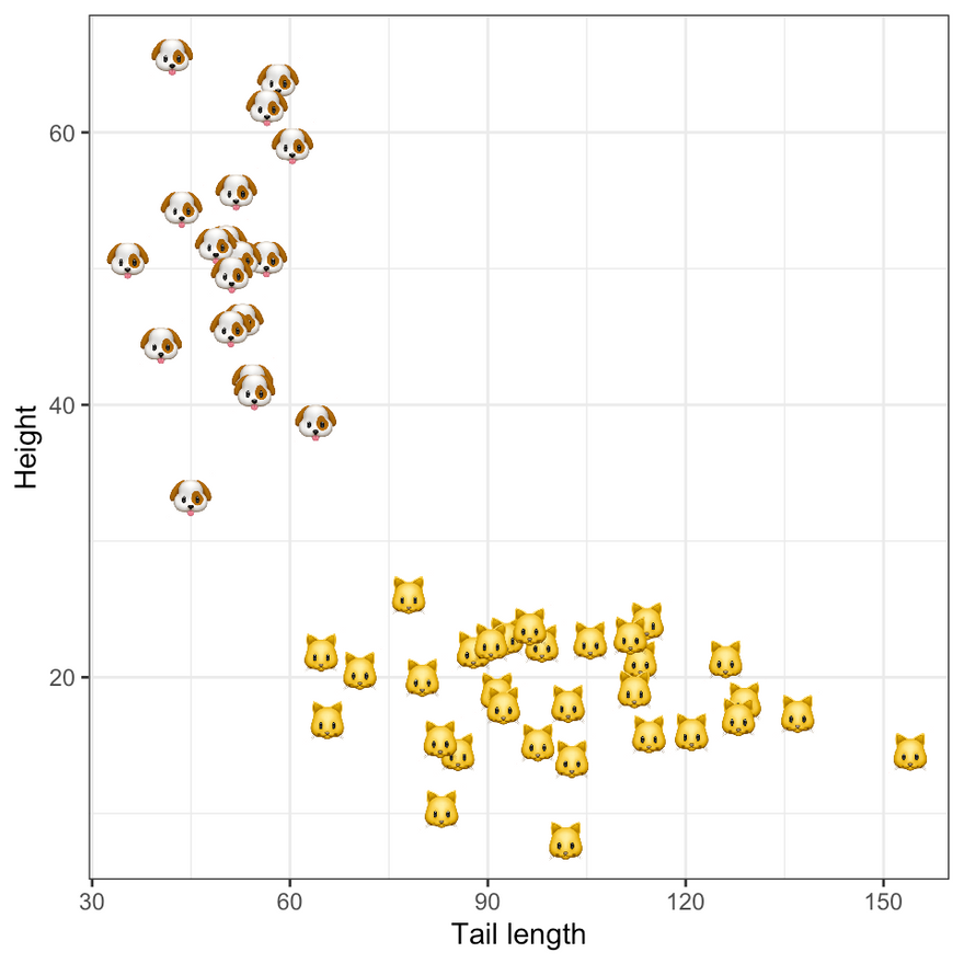
To add a little bit of life to our example we will assume that the binary labels classify samples into cats and dogs, based on their height and tail length. The figure below shows the synthetic data in the two-dimensional feature domain. Following an introduction to Bayesian Logistic Regression in the next section we will use this data to estimate our model.
Ground truth labels. Image by author.
The maths
Adding maths to articles on Medium remains a bit of a hassle, so here we will rely entirely on intuition and avoid formulas altogether. One of the perks of using Julia language is that it allows the use of Unicode characters, so the code we will see below looks almost like maths anyway. If you want to see the full mathematical treatment for a complete understanding of all the details, feel free to check out the extended version of this article on my website.
Problem setup
The starting point for Bayesian Logistic Regression is Bayes’ Theorem, which formally states that the posterior distribution of parameters is proportional to the product of two quantities: the likelihood of observing the data given the parameters and the prior density of parameters. Applied to our context this can intuitively be understood as follows: our posterior beliefs around the logistic regression coefficients are formed by both our prior beliefs and the evidence we observe (i.e. the data).
Under the assumption that individual label-feature pairs are independently and identically distributed, their joint likelihood is simply the product over their individual densities (Bernoulli). The prior beliefs around parameters are at our discretion. In practice they may be derived from previous experiments. Here we will use a zero-mean spherical Gaussian prior for reasons explained further below.
Unlike with linear regression there are no closed-form analytical solutions to estimating or maximising the posterior likelihood, but fortunately accurate approximations do exist (Murphy 2022). One of the simplest approaches called Laplace Approximation is straight-forward to implement and computationally very efficient. It relies on the observation that under the assumption of a Gaussian prior, the posterior of logistic regression is also approximately Gaussian: in particular, it this Gaussian distribution is centered around the maximum a posteriori (MAP) estimate with a covariance matrix equal to the inverse Hessian evaluated at the mode. Below we will see how the MAP and corresponding Hessian can be estimated.
Solving the problem
In practice we do not maximize the posterior directly. Instead we minimize the negative log likelihood, which is equivalent and easier to implement. The Julia code below shows the implementation of this loss function and its derivatives.
DISCLAIMER ❗️I should mention that (at the time of writing in 2021) this was the first time I program in Julia, so for any Julia pros out there: please bear with me! More than happy to hear your suggestions in the comments.
As you can see, the negative log likelihood is equal to the sum over two terms: firstly, a sum over (log) Bernoulli distributions — corresponding to the likelihood of the data — and, secondly, a (log) Gaussian distribution — corresponding to our prior beliefs.
# Loss:
function 𝓁(w,w_0,H_0,X,y)
    N = length(y)
    D = size(X)[2]
    μ = sigmoid(w,X)
    Δw = w-w_0
    l = - ∑( y[n] * log(μ[n]) + (1-y[n]) * log(1-μ[n]) for n=1:N) + 1/2 * Δw'H_0*Δw
    return l
end

# Gradient:
function ∇𝓁(w,w_0,H_0,X,y)
    N = length(y)
    μ = sigmoid(w,X)
    Δw = w-w_0
    g = ∑((μ[n]-y[n]) * X[n,:] for n=1:N)
    return g + H_0*Δw
end

# Hessian:
function ∇∇𝓁(w,w_0,H_0,X,y)
    N = length(y)
    μ = sigmoid(w,X)
    H = ∑(μ[n] * (1-μ[n]) * X[n,:] * X[n,:]' for n=1:N)
    return H + H_0
end
Since minimizing this loss function is a convex optimization problem we have many efficient algorithms to choose from in order to solve this problem. With the Hessian also at hand it seems natural to use a second-order method, because incorporating information about the curvature of the loss function generally leads to faster convergence. Here we will implement Newton’s method like so:
# Newton's Method
function arminjo(𝓁, g_t, θ_t, d_t, args, ρ, c=1e-4)
    𝓁(θ_t .+ ρ .* d_t, args...) <= 𝓁(θ_t, args...) .+ c .* ρ .* d_t'g_t
end

function newton(𝓁, θ, ∇𝓁, ∇∇𝓁, args; max_iter=100, τ=1e-5)
    # Intialize:
    converged = false # termination state
    t = 1 # iteration count
    θ_t = θ # initial parameters
    # Descent:
    while !converged && t<max_iter
        global g_t = ∇𝓁(θ_t, args...) # gradient
        global H_t = ∇∇𝓁(θ_t, args...) # hessian
        converged = all(abs.(g_t) .< τ) && isposdef(H_t) # check first-order condition
        # If not converged, descend:
        if !converged
            d_t = -inv(H_t)*g_t # descent direction
            # Line search:
            ρ_t = 1.0 # initialize at 1.0
            count = 1
            while !arminjo(𝓁, g_t, θ_t, d_t, args, ρ_t)
                ρ_t /= 2
            end
            θ_t = θ_t .+ ρ_t .* d_t # update parameters
        end
        t += 1
    end
    # Output:
    return θ_t, H_t
end
Suppose now that we have trained the Bayesian Logistic Regression model as our binary classifier using our training data and a new unlabelled sample arrives. As with any binary classifier we can predict the missing label by simply plugging the new sample into our fitted model. If at training phase we have found the model to achieve good accuracy, we may expect good out-of-sample performance. But since we are still dealing with an expected value of a random variable, we would generally like to have an idea of how noisy this prediction is.
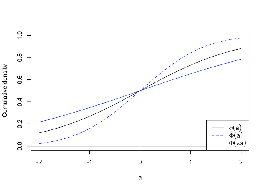
Formally, we are interested in the posterior predictive distribution, which without any further assumption is a mathematically intractable integral. It can be numerically estimated through Monte Carlo — by simply repeatedly sampling parameters from the posterior distribution — or by using what is called a probit approximation. The latter uses the finding that the sigmoid function can be well approximated by a rescaled standard Gaussian cdf (see the figure below). Approximating the sigmoid function in this way allows us to derive an analytical solution for the posterior predictive. This approach was used to generate the results in the following section.
Demonstration of the probit approximation. Image by author.
The estimates
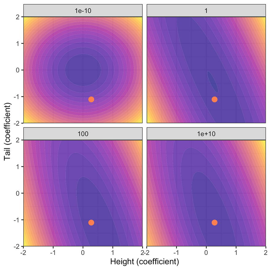
The first figure below shows the resulting posterior distribution for the coefficients on height and tail length at varying degrees of prior uncertainty. The red dot indicates the unconstrained maximum likelihood estimate (MLE). Note that as the prior uncertainty tends towards zero the posterior approaches the prior. This is intuitive since we have imposed that we have no uncertainty around our prior beliefs and hence no amount of new evidence can move us in any direction. Conversely, for very large levels of prior uncertainty the posterior distribution is centered around the unconstrained MLE: prior knowledge is very uncertain and hence the posterior is dominated by the likelihood of the data.
Posterior distribution at varying degrees of prior uncertainty σ. Image by author.
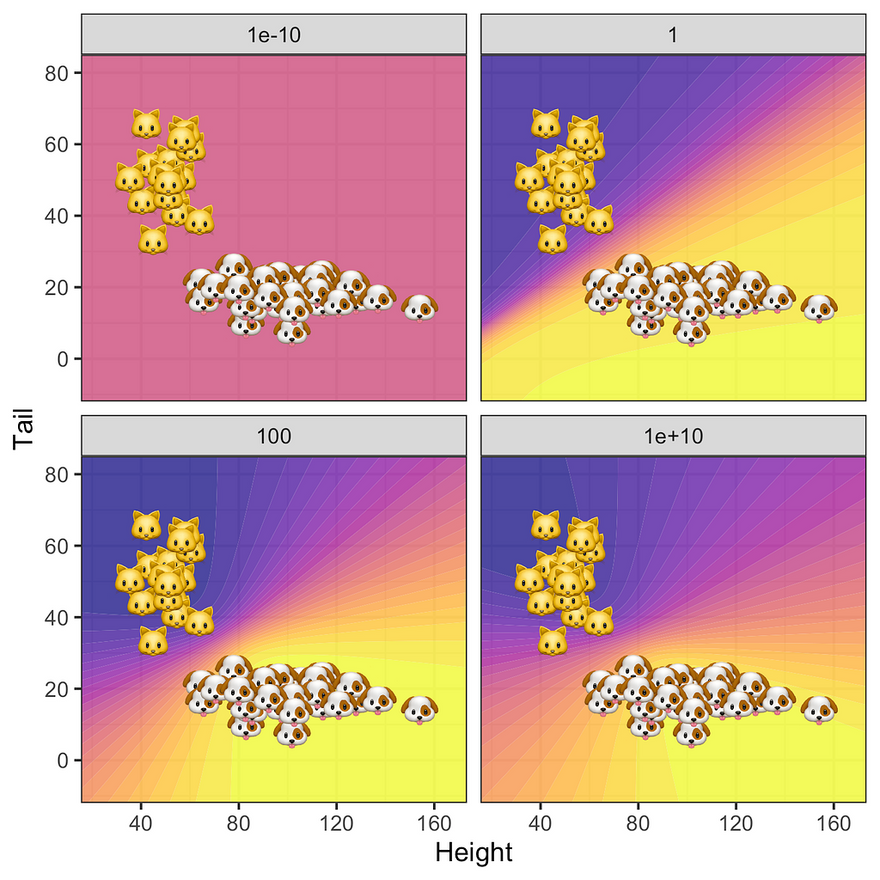
What about the posterior predictive? The story is similar: since for very low levels of prior uncertainty the posterior is completely dominated by the zero-mean prior all samples are classified as 0.5 (top left panel in the figure below). As we gradually increase uncertainty around our prior the predictive posterior depends more and more on the data: uncertainty around predicted labels is high only in regions that are not populated by samples. Not surprisingly, this effect is strongest for the MLE where we see some evidence of overfitting.
Predictive posterior distribution at varying degrees of prior uncertainty σ. Image by author.
Wrapping up
In this post we have seen how Bayesian Logistic Regression can be implemented from scratch in Julia language. The estimated posterior distribution over model parameters can be used to quantify uncertainty around coefficients and model predictions. I have argued that it is important to be transparent about model uncertainty to avoid being overly confident in estimates.
There are many more benefits associated with Bayesian (probabilistic) machine learning. Understanding where in the input domain our model exerts high uncertainty can for example be instrumental in labelling data: see for example Gal, Islam, and Ghahramani (2017) and follow-up works for an interesting application to active learning for image data. Similarly, there is a recent work that uses estimates of the posterior predictive in the context of algorithmic recourse (Schut et al. 2021). For a brief introduction to algorithmic recourse see my previous post.
As a great reference for further reading about probabilistic machine learning I can highly recommend Murphy (2022). An electronic version of the book is currently freely available as a draft. Finally, if you are curious to see the full source code in detail and want to try yourself at the code, you can check out this interactive notebook.
References
Bishop, Christopher M. 2006. Pattern Recognition and Machine Learning. springer.
Gal, Yarin, Riashat Islam, and Zoubin Ghahramani. 2017. “Deep Bayesian Active Learning with Image Data.” In International Conference on Machine Learning, 1183–92. PMLR.
Murphy, Kevin P. 2012. Machine Learning: A Probabilistic Perspective. MIT press.
— -. 2022. Probabilistic Machine Learning: An Introduction. MIT Press.
Schut, Lisa, Oscar Key, Rory Mc Grath, Luca Costabello, Bogdan Sacaleanu, Yarin Gal, et al. 2021. “Generating Interpretable Counterfactual Explanations by Implicit Minimisation of Epistemic and Aleatoric Uncertainties.” In International Conference on Artificial Intelligence and Statistics, 1756–64. PMLR.
Full article published at https://www.paltmeyer.com on November 15, 2021.

Latest comments (0)