A new tool for explainable AI

Turning a 9 (nine) into a 4 (four). Image by author.

Counterfactual explanations, which I introduced in one of my previous posts, offer a simple and intuitive way to explain black-box models without opening them. Still, as of today there exists only one open-source library that provides a unifying approach to generate and benchmark counterfactual explanations for models built and trained in Python (Pawelczyk et al. 2021). This is great, but of limited use to users of other programming languages 🥲.

Enter CounterfactualExplanations.jl: a Julia package that can be used to explain machine learning algorithms developed and trained in Julia, Python and R. Counterfactual explanations fall into the broader category of explainable artificial intelligence (XAI).

Explainable AI typically involves models that are not inherently interpretable but require additional tools to be explainable to humans. Examples of the latter include ensembles, support vector machines and deep neural networks. This is not to be confused with interpretable AI, which involves models that are inherently interpretable and transparent such as general additive models (GAM), decision trees and rule-based models.

Some would argue that we best avoid explaining black-box models altogether (Rudin 2019) and instead focus solely on interpretable AI. While I agree that initial efforts should always be geared towards interpretable models, stopping there would entail missed opportunities and anyway is probably not very realistic in times of DALL-E and Co.

Even though […] interpretability is of great importance and should be pursued, explanations can, in principle, be offered without opening the “black box.”

Wachter, Mittelstadt, and Russell (2017)

This post introduces the main functionality of the new Julia package. Following a motivating example using a model trained in Julia, we will see how easy the package can be adapted to work with models trained in Python and R. Since the motivation for this post is also to hopefully attract contributors, the final section outlines some of the exciting developments we have planned.

Counterfactuals for image data 🖼

To introduce counterfactual explanations I used a simple binary classification problem in my previous post. It involved a linear classifier and a linearly separable, synthetic data set with just two features. This time we are going to step it up a notch: we will generate counterfactual explanations MNIST data. The MNIST dataset contains 60,000 training samples of handwritten digits in the form of 28x28 pixel grey-scale images (LeCun 1998). Each image is associated with a label indicating the digit (0–9) that the image represents.

The CounterfactualExplanations.jl package ships with two black-box models that were trained to predict labels for this data: firstly, a simple multi-layer perceptron (MLP) and, secondly, a corresponding deep ensemble. Originally proposed by Lakshminarayanan, Pritzel, and Blundell (2016), deep ensembles are really just ensembles of deep neural networks. They are still among the most popular approaches to Bayesian deep learning. For more information on Bayesian deep learning see my previous post: [TDS], [blog].

Black-box models

While the package can currently handle a few simple classification models natively, it is designed to be easily extensible through users and contributors. Extending the package to deal with custom models typically involves only two simple steps:

1. Subtyping : the custom model needs to be declared as a subtype of the package-internal type AbstractFittedModel.
2. Multiple dispatch : the package-internal functions logits and probs need to be extended through custom methods for the new model type.

The code that implements these two steps can be found in the corresponding post on my own blog.

Counterfactual generators

Next, we need to specify the counterfactual generators we want to use. The package currently ships with two default generators that both need gradient access: firstly, the generic generator introduced by Wachter, Mittelstadt, and Russell (2017) and, secondly, a greedy generator introduced by Schut et al. (2021).

The greedy generator is designed to be used with models that incorporate uncertainty in their predictions such as the deep ensemble introduced above. It works for probabilistic (Bayesian) models, because they only produce high-confidence predictions in regions of the feature domain that are populated by training samples. As long as the model is expressive enough and well-specified, counterfactuals in these regions will always be realistic and unambiguous since by construction they should look very similar to training samples. Other popular approaches to counterfactual explanations like REVISE (Joshi et al. 2019) and CLUE (Antorán et al. 2020) also play with this simple idea.

The following two lines of code instantiate the two generators for the problem at hand:

generic = GenericGenerator(;loss=:logitcrossentropy) 
greedy = GreedyGenerator(;loss=:logitcrossentropy)

Explanations

Once the model and counterfactual generator are specified, running counterfactual search is very easy using the package. For a given factual (x), target class (target) and data set (counterfactual_data), simply running

generate_counterfactual(x, target, counterfactual_data, M, generic)

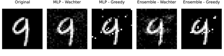
will generate the results, in this case using the generic generator (generic) for the MLP (M). Since we have specified two different black-box models and two different counterfactual generators, we have four combinations of a model and a generator in total. For each of these combinations I have used the generate_counterfactual function to produce the results in Figure 1.

In every case the desired label switch is in fact achieved, but arguably from a human perspective only the counterfactuals for the deep ensemble look like a four. The generic generator produces mild perturbations in regions that seem irrelevant from a human perspective, but nonetheless yields a counterfactual that can pass as a four. The greedy approach clearly targets pixels at the top of the handwritten nine and yields the best result overall. For the non-Bayesian MLP, both the generic and the greedy approach generate counterfactuals that look much like adversarial examples: they perturb pixels in seemingly random regions on the image.

Figure 1: Counterfactual explanations for MNIST: turning a nine (9) into a four (4). Image by author.

Language interoperability 👥

The Julia language offers unique support for programming language interoperability. For example, calling R or Python is made remarkably easy through RCall.jl and PyCall.jl, respectively. This functionality can be leveraged to use CounterfactualExplanations.jl to generate explanations for models that were developed in other programming languages. At this time there is no native support for foreign programming languages, but the following example involving a torch neural network trained in R demonstrates how versatile the package is. The corresponding example involving PyTorch is analogous and therefore omitted, but available here.

Explaining a model trained in R

We will consider a simple MLP trained for a binary classification task. As before we first need to adapt this custom model for use with our package. The code below the two necessary steps — sub-typing and method extension. Logits are returned by the torch model and copied from the R environment into the Julia scope. Probabilities are then computed inside the Julia scope by passing the logits through the sigmoid function.

using Flux
using CounterfactualExplanations, CounterfactualExplanations.Models
import CounterfactualExplanations.Models: logits, probs # import functions in order to extend

# Step 1)
struct TorchNetwork <: Models.AbstractFittedModel
    nn::Any
end

# Step 2)
function logits(M::TorchNetwork, X::AbstractArray)
  nn = M.nn
  y = rcopy(R"as_array($nn(torch_tensor(t($X))))")
  y = isa(y, AbstractArray) ? y : [y]
  return y'
end
function probs(M::TorchNetwork, X::AbstractArray)
  return σ.(logits(M, X))
end
M = TorchNetwork(R"model")

Compared to models trained in Julia, we need to do a little more work at this point. Since our counterfactual generators need gradient access, we essentially need to allow our package to communicate with the R torch library. While this may sound daunting, it turns out to be quite manageable: all we have to do is respecify the function that computes the gradient with respect to the counterfactual loss function so that it can deal with the TorchNetwork type we defined above. The code below implements this.

import CounterfactualExplanations.Generators: ∂ℓ
using LinearAlgebra

# Countefactual loss:
function ∂ℓ(
    generator::AbstractGradientBasedGenerator, 
    counterfactual_state::CounterfactualState) 
  M = counterfactual_state.M
  nn = M.nn
  x′ = counterfactual_state.x′
  t = counterfactual_state.target_encoded
  R"""
  x <- torch_tensor($x′, requires_grad=TRUE)
  output <- $nn(x)
  loss_fun <- nnf_binary_cross_entropy_with_logits
  obj_loss <- loss_fun(output,$t)
  obj_loss$backward()
  """
  grad = rcopy(R"as_array(x$grad)")
  return grad
end

That is all the adjustment needed to use CounterfactualExplanations.jl for our custom R model. Figure 2 shows a counterfactual path for a randomly chosen sample with respect to the MLP trained in R.

Figure 2: Counterfactual path using the generic counterfactual generator for a model trained in R. Image by author.

We need you! 🫵

The ambition for CounterfactualExplanations.jl is to provide a go-to place for counterfactual explanations to the Julia community and beyond. This is a grand ambition, especially for a package that has so far been built by a single developer who has little prior experience with Julia. We would therefore very much like to invite community contributions. If you have an interest in trustworthy AI, the open-source community and Julia, please do get involved! This package is still in its early stages of development, so any kind of contribution is welcome: advice on the core package architecture, pull requests, issues, discussions and even just comments below would be much appreciated.

To give you a flavour of what type of future developments we envision, here is a non-exhaustive list:

1. Native support for additional counterfactual generators and predictive models including those built and trained in Python or R.
2. Additional datasets for testing, evaluation and benchmarking.
3. Improved preprocessing including native support for categorical features.
4. Support for regression models.

Finally, if you like this project but don’t have much time, then simply sharing this article or starring the repo on GitHub would also go a long way.

Further reading 📚

If you’re interested in learning more about this development, feel free to check out the following resources:

• Package docs: [stable], [dev].
• Contributor’s guide.
• GitHub repo.

Thanks 💐

Lisa Schut and Oscar Key — corresponding authors of Schut (2021) — have been tremendously helpful in providing feedback on this post and answering a number of questions I had about their paper. Thank you!

References

Antorán, Javier, Umang Bhatt, Tameem Adel, Adrian Weller, and José Miguel Hernández-Lobato. 2020. “Getting a Clue: A Method for Explaining Uncertainty Estimates.” arXiv Preprint arXiv:2006.06848.

Joshi, Shalmali, Oluwasanmi Koyejo, Warut Vijitbenjaronk, Been Kim, and Joydeep Ghosh. 2019. “Towards Realistic Individual Recourse and Actionable Explanations in Black-Box Decision Making Systems.” arXiv Preprint arXiv:1907.09615.

Lakshminarayanan, Balaji, Alexander Pritzel, and Charles Blundell. 2016. “Simple and Scalable Predictive Uncertainty Estimation Using Deep Ensembles.” arXiv Preprint arXiv:1612.01474.

LeCun, Yann. 1998. “The MNIST Database of Handwritten Digits.” Http://Yann. Lecun. Com/Exdb/Mnist/.

Pawelczyk, Martin, Sascha Bielawski, Johannes van den Heuvel, Tobias Richter, and Gjergji Kasneci. 2021. “Carla: A Python Library to Benchmark Algorithmic Recourse and Counterfactual Explanation Algorithms.” arXiv Preprint arXiv:2108.00783.

Rudin, Cynthia. 2019. “Stop Explaining Black Box Machine Learning Models for High Stakes Decisions and Use Interpretable Models Instead.” Nature Machine Intelligence 1 (5): 206–15.

Schut, Lisa, Oscar Key, Rory Mc Grath, Luca Costabello, Bogdan Sacaleanu, Yarin Gal, et al. 2021. “Generating Interpretable Counterfactual Explanations by Implicit Minimisation of Epistemic and Aleatoric Uncertainties.” In International Conference on Artificial Intelligence and Statistics, 1756–64. PMLR.

Wachter, Sandra, Brent Mittelstadt, and Chris Russell. 2017. “Counterfactual Explanations Without Opening the Black Box: Automated Decisions and the GDPR.” Harv. JL & Tech. 31: 841.

Originally published at https://www.paltmeyer.com on April 20, 2022.