When you want to convince people that Julia is the best language for some task, some are easily swayed by the beautiful syntax, rank polymorphism, and flirtations with functional programming. In all honesty, those people need little convincing. Others want to see hard numbers!
Here's a very small demo that shows how Julia can outperform any traditional language: computing polynomials.
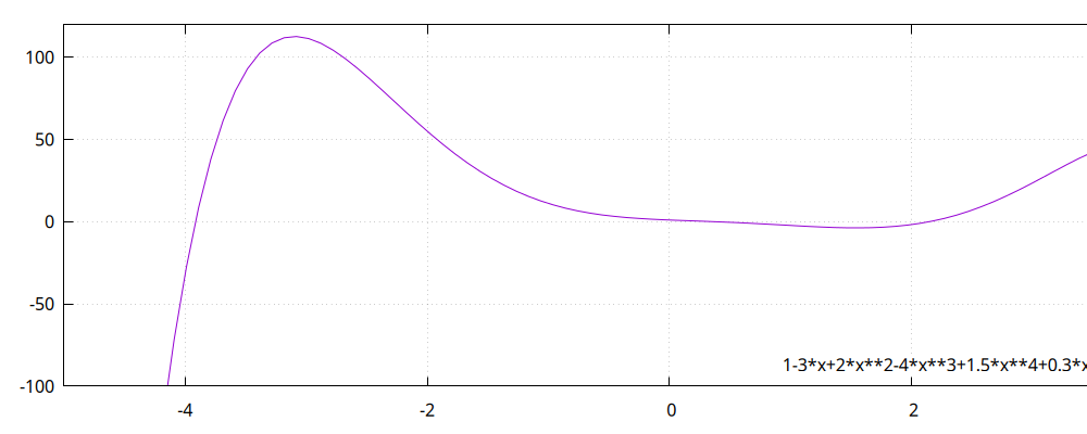
Suppose we have a function described by
where we have the coefficients stored in some dense vector.
struct Polynomial{T}
    c::Vector{T}
end
We can evaluate this function as follows:
function (f::Polynomial{T})(x::T) where T<:Number
    result = f.c[1]
    xpow = x
    for c in f.c[2:end-1]
        result += xpow * c
        xpow *= x
    end
    result + xpow * f.c[end]
end
This is very much how you would implement such a function in most other languages. In Julia however, we can do something much nicer: generate a function.
function expand(f::Polynomial{T}) where T<:Number
    :(function (x::$T)
        r = $(f.c[1])
        xp = x
        $((:(r += xp*$c; xp*=x) for c in f.c[2:end-1])...)
        r + xp * $(f.c[end])
    end)
end
Now, when we expand(f), say we have f = Polynomial(1.0, 0.5, 0.333, 0.25) the generated function will look as follows:
:(function (x::Float64,)
      r = 1.0
      xp = x
      begin
          r += xp * 0.5
          xp *= x
      end
      begin
          r += xp * 0.333
          xp *= x
      end
      r + xp * 0.25
  end)
To run this, we say f_unroll = eval(expand(f)). Not only does this run much faster than our previous loopy implementation, it even outperforms C++ (GCC at -O3) by more than a factor of two (depending on your machine). The reason is that we have no loop in our generated code, and more importantly, we are not accessing any memory. We have done something that a C++ programmer wouldn't dream of doing: write a code generator, compile the specialised code, and fly to the moon!
A completely literate and Documentered implementation of this demo can be found here.
Edit: Thanks to Nicos Pitsianis for point out to me that there is a more efficient method called Horner's method. This method applies to both Julia and C++ implementations, reducing the amount of multiplications needed. Using this method reduces the difference between Julia and C++ a little bit, but increasing the order of the polynomial grows it back again.

Latest comments (5)
I've tried to reproduce the benchmarks of all three versions of the algorithm, you presented in "A completely literate and Documentered implementation ...". There are three variants presented (variant 2 and 3 are shown in the post above).
My environment is Julia 1.9.1 on Apple M1. I've used the
@benchmark-macro from theBenchmarkTools-package. This macro calls the expression to be measured several hundred times in order to obtain a reliable statistics. So there is no need for the functionstest_f1,test_f2andtest_f3. I've basically evaluated the expression inside these functions (which is more or less equivalent to calling these functions withn = 1).This resulted in the following run times in ms for evaluating 100,000 arguments with variants 1-3: 6.35/2.30/0.15 (original in the table below).
Then I tried to insulate the pure algorithm a bit more, eliminating other effects which may degrade run time. There are basically two aspects:
fand its argumentsxs) isn't recommended for the Julia compiler. It is better to pass them as function arguments of to declare them asconst. It did the latter.LinRangefor the arguments uses lazy evaluation. I.e. the numbers are only created when needed for evaluation. So I applied acollecton them in order to pre-allocate all arguments.Using
constvalues is a huge improvement for variant 2. So the speedup from variant 2 to 3 gets much smaller (but still is great).The following table shows all results and the speedups based on these numbers. For comparison I've also added the numbers of the Julia standard function
evalpoly.Note that Julia
Basehas a function for evaluating a polynomial given by coefficients:Base.Math.evalpoly:docs.julialang.org/en/v1/base/math...
On the other hand, when you're willing to preprocess the polynomial (prior to evaluating it lots of times), techniques that may be faster than
evalpolyare possible.Shouldn't it be faster if you used Horner's rule to evaluate the polynomial? It would require a single multiplication (instead of two) and a single addition per coefficient.
The unrolled code will also be shorter.
Thanks for the tip! I'll add this to the code.
Very interesting. Also something that most are unaware of. i.e literate programming. 👍