Random forest, Shapley values and multicollinearity

Linear statistical models are great for many use-cases since they are easy to use and easy to interpret. Specifically, linear models can use features (also known as independent variables, predictors or covariates) to predict an outcome (also known as dependent variables).

In a linear model, a higher coefficient for a feature, the more a feature played a role in making a prediction. However, when variables in a regression model are correlated, these conclusions don't hold anymore.

One way to solve this is to use clustering techniques such as principal component analysis (PCA) (Dormann et al., 2012). With PCA, latent clusters are automatically determined. Unfortunately, these latent clusters now became, what I would like to call, magic blobs. Proponents of these techniques could say: "But we know that there is an underlying variable which causes our effect, why can't this variable be the same as the cluster that we found?" Well, because these blobs are found in the data and not in the real-world.

To link these blobs (officially, clusters) back to the real-world, one can try to find the features closes to the blobs in one way or another, but this will always introduce bias. Another approach is to drop features which are highly correlated and expected to be less important.

Some say that random forests combined with Shapley values can deal with collinearity reasonably well. This is because the random forest can find complex relations in the data and because Shapley values are based on mathematically proven ideas. Others say that the Shapley values will pick one of the correlated features and ignore the others. In this post, I aim to simulating collinear data and see how good the conclusions of the model are.

Simulating data

begin
    using CairoMakie
    using DataFrames: Not, DataFrame, select
    using Distributions: Normal
    using LightGBM.MLJInterface: LGBMRegressor
    using MLJ: fit!, machine, predict
    using Random: seed!
    using Shapley: MonteCarlo, shapley
    using StableRNGs: StableRNG
    using Statistics: cor, mean
end

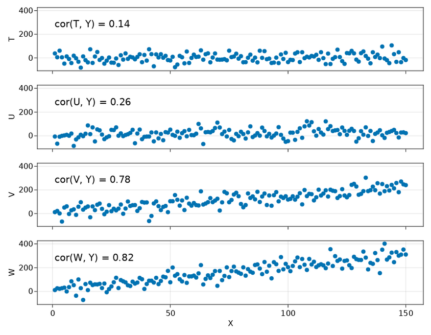
y_true(x) = 2x + 10;
y_noise(x, coefficient) = coefficient * y_true(x) + rand(Normal(0, 40));
indexes = 1.0:150.0;
r2(x) = round(x; digits=2);

df = let
    seed!(0)
    X = indexes
    T = y_noise.(indexes, 0)
    U = y_noise.(indexes, 0.05)
    V = y_noise.(indexes, 0.7)
    W = y_noise.(indexes, 1)
    Y = y_noise.(indexes, 1)

    DataFrame(; X, T, U, V, W, Y)
end;

Fitting a model

For the LGBM regressor, I've set some hyperparameters to lower values because the default parameters are optimized for large datasets.

function regressor()
    kwargs = [
        :num_leaves => 9,
        :max_depth => 3,
        :min_data_per_group => 2,
        :learning_rate => 0.5
    ]
    return LGBMRegressor( ; kwargs...)
end;

function fit_model(df::DataFrame)
    X = select(df, Not([:X, :Y]))
    y = df.Y
    m = fit!(machine(regressor(), X, y))
    return X, y, m
end;

To get an idea of what the model is doing, we can plot the predictions on top of the data.

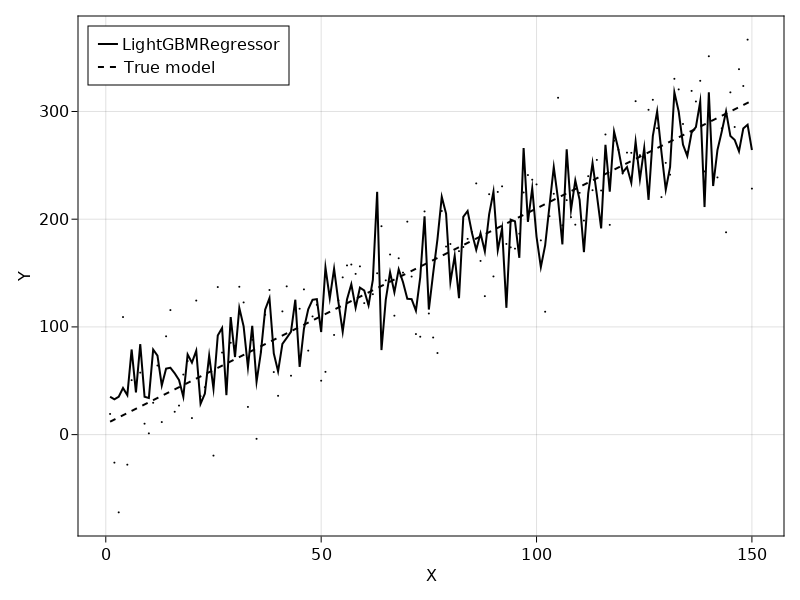
My main worry after seeing this is how we can avoid overfitting random forests on our data. Intuitively, it makes sense that the model overfits due to it's high flexibility combined with few samples. Of course, not all real-world phenomenons are linear, but it seems that the model is spending too much effort on fitting noise. Luckily, approaches such as (nested) cross-validation can estimate how well a model will generalize.

Anyway, I'm digressing. Back to the original problem of whether we can infer anything from the non-linear model about feature importance.

Shapley values

Shapley values are based on a theory by Shapley (1953). The goal of these values is to estimate how much each feature has contributed to the prediction. One way to do this is by changing the input for a feature while keeping all other feature inputs constant and seeing how much the output changes. This repeated sampling is called the Monte Carlo method. We can aggregate the Monte Carlo results to estimate how much a feature contributes to the outcome.

function shapley_values(df::DataFrame)
    X, y, m = fit_model(df)
    mc = MonteCarlo(1024)
    return shapley(x -> predict(m, x), mc, X)
end;

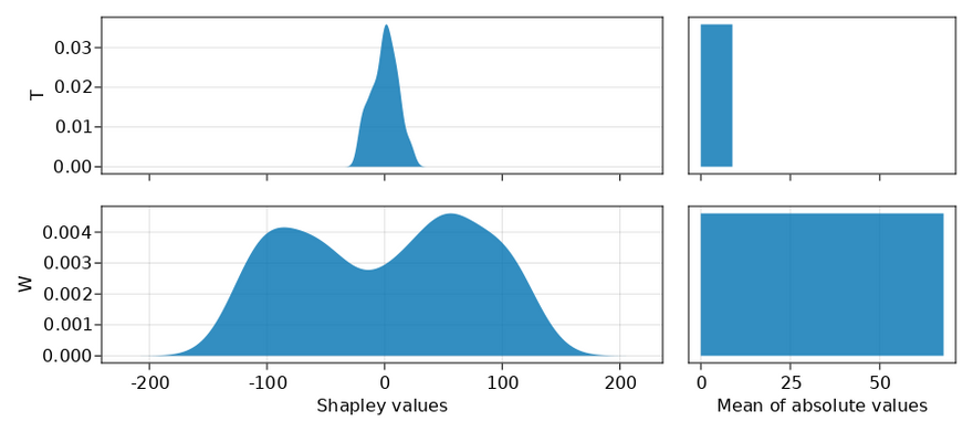
As a simple check, let's first see what happens if we only pass the dataset with X, T, W and Y. Because T has no relation to the outcome Y and W has a strong relation to the outcome Y, we expect that T gets a low score and W gets a high score.

In the plot below, I've shown all the Shapley values from the Monte Carlo simulation on the left and aggregated them on the right. As expected, the plots on the right clearly show that W has a greater contribution.

As a sidenote, usually people only show the plot on the right (mean of absolute values) when talking about Shapley values, but I think it is good to have the one on the left (Shapley values) too to give the full picture.

Now, it's time for the final test: do Shapley values give apropriate credit to correlated features? We check this by passing all the features instead of only X, T, W and Y.

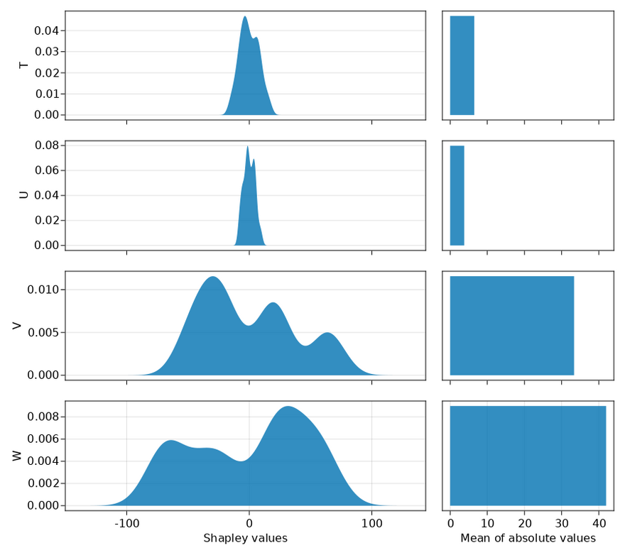
Based on this outcome, I would say that Shapley values do a pretty good job in combination with the LightGBM model. The values T, U, V, W are ordered by their correlation with the outcome (and each other). As expected, features lower in the plot get a higher mean of absolute values, that is, feature importance. However, basing scientific conclusions on these outcomes may be deceptive because it's likely that there is a high variance on the reported feature importances. The main risk is here is that the model didn't properly fit resulting in incorrect outcomes. Another risk is that the overfitted model generalizes poorly. Both risks also hold for linear models, so I guess it's just the best we have.

Built with Julia 1.8.0 and

CairoMakie 0.8.13
DataFrames 1.3.4
Distributions 0.25.67
LightGBM 0.5.2
MLJ 0.18.4
Shapley 0.1.1
StableRNGs 1.0.0 

To run this blog post locally, open this notebook with Pluto.jl.