
To me, it is still unclear what exactly is the difference between Frequentist and Bayesian statistics. Most explanations involve terms such as "likelihood", "uncertainty" and "prior probabilities". Here, I'm going to show the difference between both statistical paradigms by using a coin flipping example. In the examples, the effect of showing more data to both paradigms will be visualised.
Generating data
Lets start by generating some data from a fair coin flip, that is, the probability of heads is 0.5.
begin
    import CairoMakie

    using AlgebraOfGraphics: Lines, Scatter, data, draw, visual, mapping
    using Distributions
    using HypothesisTests: OneSampleTTest, confint
    using StableRNGs: StableRNG
end
n = 80;
p_true = 0.5;
is_heads = let
    rng = StableRNG(15)
    rand(rng, Bernoulli(p_true), n);
end;
To give some intuition about the sample, the first six elements of is_heads are:
is_heads[1:6]
6-element Vector{Bool}:
 1
 1
 1
 0
 0
 1
Calculate probability estimates
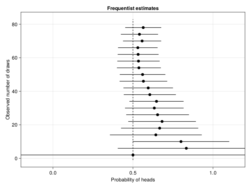
The Frequentist estimate for a one sample t-test after seeing nnn samples can be calculated with
function frequentist_estimate(n)
    t_result = OneSampleTTest(is_heads[1:n])
    middle = t_result.xbar
    lower, upper = confint(t_result)
    return (; lower, middle, upper)
end;
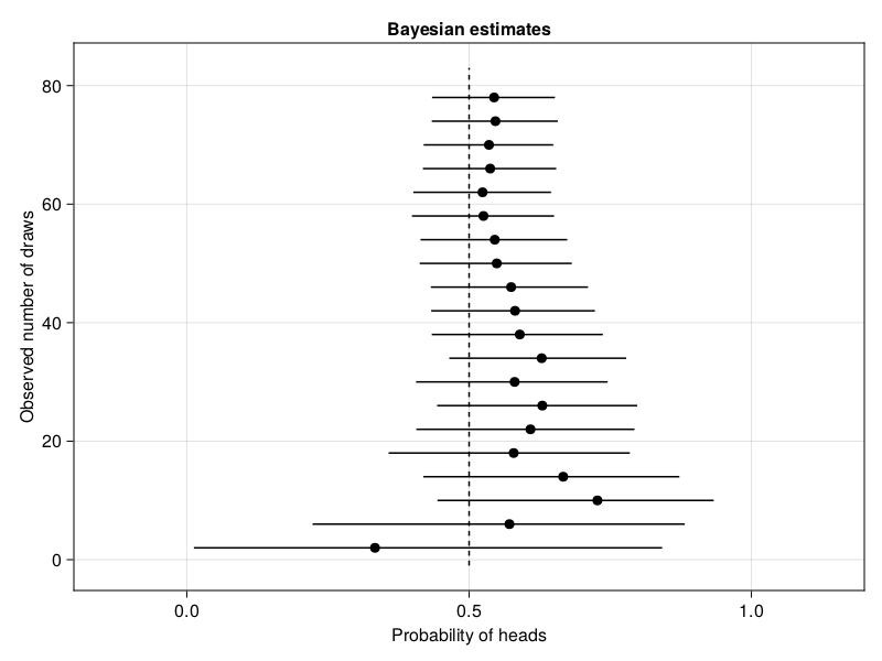
For the Bayesian estimate, we can use the closed-form solution (https://turing.ml/dev/tutorials/00-introduction/). A closed-form solution is not available for many real-world problems, but quite useful for this example.
closed_form_prior = Beta(1, 1);
function update_belief(k)
    heads = sum(is_heads[1:k-1])
    tails = k - heads
    updated_belief = Beta(closed_form_prior.α + heads, closed_form_prior.β + tails)
    return updated_belief
end;
beliefs = [closed_form_prior; update_belief.(1:n)];
function bayesian_estimate(n)
    distribution = beliefs[n]
    q(x) = quantile(distribution, x)
    lower = q(0.025)
    middle = mean(distribution)
    upper = q(0.975)
    return (; lower, middle, upper)
end;
Now we can write a function to plot the estimates:
function plot_estimates(estimate_function; title="")
    draws = 2:4:80
    estimates = estimate_function.(draws)
    middles = [t.middle for t in estimates]
    lowers = [t.lower for t in estimates]
    uppers = [t.upper for t in estimates]
    df = (; draws, estimates, P=middles)
    layers = data(df) * visual(Scatter)
    df_middle = (; P=fill(0.5, length(draws) + 2), draws=[-1; draws; 83])
    layers += data(df_middle) * visual(Lines) * visual(linestyle=:dash)
    for (n, lower, upper) in zip(draws, lowers, uppers)
        df_bounds = (; P=[lower, upper], draws=[n, n])
        layers += data(df_bounds) * visual(Lines)
    end

    axis = (; yticks=0:20:80, limits=((-0.2, 1.2), nothing), title)
    map = mapping(:P => "Probability of heads", :draws => "Observed number of draws")
    draw(layers * map; axis)
end;
And plot the Frequentist and Bayesian estimates:
plot_estimates(frequentist_estimate; title="Frequentist estimates")
plot_estimates(bayesian_estimate; title="Bayesian estimates")
Conclusion
Based on these plots, we can conclude two things. Firstly, the Bayesian approach provides better estimates for small sample sizes. The Bayesian approach successfully uses the fact that a probability should be between 0 and 1, which was given to the model via the Beta(1, 1) prior. For increasingly larger sample sizes, the difference between both statistical paradigms vanish in this situation. Secondly, collecting more and more samples until the result is significant is dangerous. This approach is called optional stopping. Around 10 samples, the frequentist' test would conclude that the data must come from a distribution with a mean higher than 0.5, whereas we know that this is false. Cumming (2011) calls this the "dance of the p-values".
EDIT: Christopher Rowley pointed out that it would be more fair to run a frequentist BinomialTest since that will output a confidence interval in [0, 1].
Built with Julia 1.8.0 and
AlgebraOfGraphics 0.6.11
CairoMakie 0.8.13
Distributions 0.25.70
HypothesisTests 0.10.10
StableRNGs 1.0.0
To run this blog post locally, open this notebook with Pluto.jl.

Oldest comments (5)
Very nice article. The difference is in terms of interpretation, but can be meaningful in the way you model stuff. The frequentist is assuming that you want to calculate the probability of observing a sample
xgiven that the real paramater of the model is theta.Hence, it makes the assumption that theta is deterministic, and hence, making probabilistic statement regarding theta are non-sense.
The Baysian always presumes a distribution for the parameter.
The two can be somewhat reconciled via what one would call a hierarchical model. Hence, the frequentist would also assume theta to be random, and another parameter (gamma) to be the deterministic one. This is similar to the Bayesian modeling.
The main weakness I see in the Bayesian interpretation comes from the "prior as a degree of belief", which is just bs to me. The weakness in frequentism is assume that parameters are deterministic, when in reality they mostly are not.
Lovely article, and I'm just reading up on these topics. My question is regarding the Conclusion section, it says "around 30 samples..." and looking at the frequentist plot, I can see 0.5 being firmly within the confidence interval the whole process. Am I missing something? Did the comment refer to a different random seed?
(also, it seems Turing.jl isn't used, so it doesn't have to be imported. The Bayesian calculation is similar to one in Turing documentation on the section of calculation without Turing).
Thank you! You are right.
I've switched from loading
Turing.jlto onlyDistributions.jl. Regarding the confidence interval, I was using aRandom.seed!instead of theStableRNG, so that broke things when I updated this post to Julia 1.8. It's fixed now.Nice article. Just one thing, since you are estimating a probability, a
BinomialTestis more appropriate than aOneSampleTTest. This will output a confidence interval in [0,1] and be more accurate, especially at lower numbers of samples. This addresses the first part of your conclusion.Thank you. I didn't know that and added a comment in the article.