Steven Siew

Posted on Apr 10, 2023 • Updated on Apr 28, 2023

Understanding Markov Chain Monte Carlo with Metropolis Algorithm

#mcmc #mathematics #bayesian

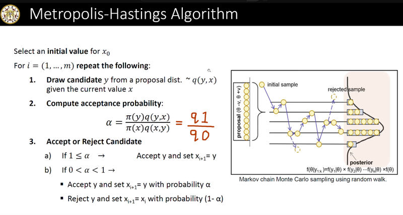
What is Markov Chain Monte Carlo

Markov Chain Monte Carlo is a method by which (additional) samples can be generated (from the last sample) such that the probability density of samples (in total) is proportional to a known function.

What Markov Chain Monte Carlo is used for is parameter estimation (such as means, variances, expected values) and exploration of the posterior distribution of Bayesian models.

Another way to think of Markov Chain Monte Carlo is this:

Imagine a process which produces data, for example, a bias coin producing a series of coin toss results.

H,T,T,H,T,T,T,T,H,T

What Markov Chain Monte Carlo does is to take the result of the coin toss and produce a series of parameter (or parameters) which could be the ACTUAL parameter of the bias coin. The more likely the parameter to be the ACTUAL PARAMETER, the more often it is produced by the Markov Chain Monte Carlo simulation.

So what you need to know is this:

ACTUAL PARAMETER in a process produces the data (a sequence of datum) in an experiment

We collect the actual data and feed it to Markov Chain Monte Carlo Simulation so that it produces a list of Parameter candidates where the most common parameter candidate is the one to be most likely to be the ACTUAL PARAMETER.

What is Metropolis Algorithm

In 1952, Arianna Rosenbluth together with her husband Marshall Rosenbluth worked on what is now known as the Metropolis Hastings algorithm.

They worked on (aka used) the supercomputer MANIAC on Los Alamos National Laboratory in 1952.

Metropolis Hastings algorithm is the very first MCMC algorithm.

https://youtu.be/evyKPVS_M7E
She's a MANIAC, MANIAC on the computing floor
And she's computing like she's never computed before

If you need to read a paper on Metropolis Hastings algorithm, you can get the PDF paper here

https://link.springer.com/article/10.3758/s13423-016-1015-8

I am sorry that I ask you to read the paper above but they can explain MCMC (Markov Chain Monte Carlo) better than I can.

MCMC is a form of Bayesian inference.

Bayesian inference uses the information provided by observed data about a (set of) parameter(s), formally the likelihood, to update a prior state of beliefs about a (set of) parameter(s) to become a posterior state of beliefs about a (set of) parameter(s).

If the above sounds like gobbledygook to you then as a newbie you are NOT ALONE.

What it means is that

You have an idea about the process that generates results in an experiment.
The process have a set of ACTUAL parameters with ACTUAL (but unknown) values.
You have a vague idea about the values of the parameters BEFORE you start the experiment. This idea is called "prior parameter values" or simply as "prior".
You perform the experiment (or ask someone else to do so)
After the experiment, you feed the data from the experiment to MCMC
Then you have to tell MCMC how to calculate the likelihood of obtaining a specific datum from a specific set of parameter values. This is done by providing MCMC with the likelihood function.
The MCMC tool returns the result which is the most likely values of the parameters. This result is called "posterior parameter values" or simply as "posterior"

So, newbie, what this means is that

For MCMC to tell you what the parameter values are, you must first tell MCMC what you THINK the parameter values are BEFORE you start the experiment. Yes, I know it sounds CRAZY!!!

Because the only reason you perform the experiment is to find out the value of the parameters in the first place. What if you know NOTHING about the value of the parameter? What do you tell MCMC? "Hello MCMC, I know nothing about the possible value of the parameter. Let me perform the experiment first, then I can tell you what the values of the parameter might be." But NO. MCMC wants you to tell it what you know about the value of the parameter BEFORE you start the experiment.

Welcome to the crazy world of Bayesian Inference.

Watch a video about Markov Chain Monte Carlo

Please watch this video about Markov Chain Monte Carlo

https://youtu.be/Qqz5AJjyugM

Metropolis Hastings Algorithm

Step 1 : Gather the data from an experiment.

An experiment can be anything. It can be as simple as asking all the students in a high school class to step on a weight scale and record down the weight of each student in kilograms.

data[1] = 55.8 kg
.
.
.
data[10] = 63.5 kg

Step 2 : Come up with a model process which produces the data

The Markov Chain Monte Carlo is NOT a magic tool. It cannot give you a model process. Instead you have to come up with the model process by yourself. You have to use your knowledge, the current scientific knowledge or even pure dumb guesses to come up with a process model.

Say your model process is that

The weight of each student is generated by a Gaussian/Normal Distribution with the mean μ (aka mu) and the standard deviation σ (aka sigma)

In Turing.jl it would look something like this

data[k] ~ Normal(μ,σ)

Step 3 : Pick a random starting value for the parameter

In this step, we need to inform MCMC of our belief about the vague values of our parameters μ (mu) and σ (sigma) before the EXPERIMENT starts.

Here for μ (mu), we need to express our real world knowledge into a mathematical distribution.

We know the lightest person on earth (via www.google.com) is about 6.0 kg and the heaviest person on earth is about 600.0 kg (,remember I said VAGUE values). So we can say

Our belief about the average weight μ (mu) is represented by

prior_μ_distr = Distributions.Uniform(6.0,600.0)

But our daily common sense says most people weights about 60.0 kg so we can also express it as:

prior_μ_distr = Distributions.Normal(60, 10)

And for σ (sigma), we know that it cannot be NEGATIVE. So we can use the Exponential distribution because it is always positive.

prior_μ_distr = Distributions.Normal(60, 10)
prior_σ_distr = Distributions.Exponential(20)
p_μ[1] = rand(prior_μ_distr)
p_σ[1] = rand(prior_σ_distr)

or you can pick any value out of the thin air

prior_μ_distr = Distributions.Uniform(30,90)
prior_σ_distr = Distributions.Uniform(0,50)
p_μ[1] = 40.0
p_σ[1] = 5.0

Step 4 : Pick a range for the parameter(s)

One of the reason, we need Upper Bound and Lower Bound (and JumpingWidth) is to generate the standard deviation for jumping distance.

standard_deviation_for_jumping_distance is
JumpingWidth*(μ_ub-μ_lb)

Later in the Module SimpleMCMC, we don't need Upper Bound and Lower Bound because we can automatically generate a standard deviation to determine the jumping distance.

μ_lb = 30       # Lower bound
μ_ub = 90       # Upper bound

σ_lb = 0        # Lower bound
σ_ub = 50       # Upper bound

Step 5 : get a candidate for new parameter

p_μ_current = p_μ[1]
p_σ_current = p_σ[1]
JumpingWidth = 0.01
p_μ_new = rand(  Normal( p_μ_current , JumpingWidth*(μ_ub-μ_lb) )  )
p_σ_new = rand(  Normal( p_σ_current , JumpingWidth*(σ_ub-σ_lb) )  )

Step 6 : Create a function to determine the probability that the data collected is a result of a particular parameter

# The likelihood function which returns the probability,
# given a fixed mu and a fixed sigma, of generating 
# the sequence of datapoints
function likelihood(data::Vector,mu::Real,sigma::Real)
    numofdatapoints = length(data)
    result=1.0
    for k = 1:numofdatapoints
        result *= pdf(Normal(mu, sigma),data[k])
    end
    return result
end

where

? pdf

pdf(d::Distribution{ArrayLikeVariate{N}}, x) where {N}

Evaluate the probability density function of d at every element in a collection x.

Step 7 : Starting at parameter[1] , generate a fix number of new parameters using the following algorithm:

Generate a candidate.
Find the prior for the current_parameter. (priorμ0 and priorσ0)
Find the prior for the candidate_for_new_parameter. (priorμ1 and priorσ1)
Find the likelihood of current_parameter.
Find the likelihood of candidate_for_new_parameter.
Calculate q0 and q1.
If q1 > q0 then select the candidate_for_new_parameter. Otherwise generate a random number between 0 and 1.
If the random number is less than q1/q0 then select the candidate_for_new_parameter otherwise select current_parameter

n_samples = 1_000_000

for i in 2:n_samples
    # Generate a candidate. 
    p_μ_new = rand(  Normal( p_μ[i-1] , JumpingWidth*(μ_ub-μ_lb) )  )
    p_σ_new = rand(  Normal( p_σ[i-1] , JumpingWidth*(σ_ub-σ_lb) )  )

    priorμ0 = Distributions.pdf(prior_μ_distr,p_μ[i-1])
    priorσ0 = Distributions.pdf(prior_σ_distr,p_μ[i-1])    

    priorμ1 = Distributions.pdf(prior_μ_distr,p_μ_new)
    priorσ1 = Distributions.pdf(prior_σ_distr,p_σ_new)

    # Find the likelihood of current_parameter
    L0 = likelihood(data, p_μ[i-1], p_σ[i-1])

    # Calculate q0
    q0 = L0 * priorμ0 * priorσ0

    # Find the likelihood of candidate_for_new_parameter.
    L1 = likelihood(data, p_μ_new, p_σ_new)

    # Calculate q1
    q1 =  L1 * priorμ1 * priorσ1

    if rand() < q1/q0  # Then jump to the NEW POSITION
        p_μ[i] = p_μ_new
        p_σ[i] = p_σ_new
    else  # Stick with the CURRENT POSITION
        p_μ[i] = p_μ[i-1]
        p_σ[i] = p_σ[i-1]
    end
end

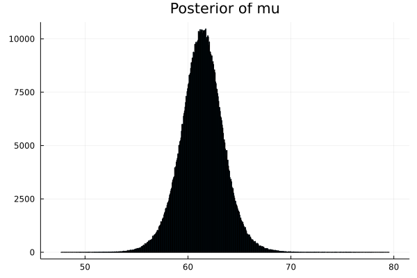
Step 8 : Now we have the array of parameters. We can plot the density graphs.

array of p_μ
array of p_σ

# Next we need to display the histogram of the array p
# this is the shape of the posterior produced by MCMC
histogram(p_μ,legend=false,title="Posterior of mu") |> display
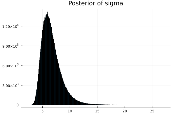
histogram(p_σ,legend=false,title="Posterior of sigma") |> display

Here is a diagram from a youtube video that illustrate what we are trying to do.

Simple Julia implementation of Metropolis Algorithm

using Distributions
using StatsPlots

# Here are the weights of the students (in kilograms) in a classrom
# Assuming the weight of the students are generated by a biological
# process with a normal distribution with mean μ and standard dev σ
# find the posterior distribution of those two parameters
data = [ 55.8, 64.1, 61.2, 55.2, 58.0, 69.8, 53.2, 70.0, 63.3, 63.5 ]

# define our prior for μ as a normal centered on 60 ( required for MCMC )
prior_μ_distr = Distributions.Normal(60, 10)
prior_μ(p) = Distributions.pdf(prior_μ_distr,p)
μ_lb = 30       # Lower bound
μ_ub = 90       # Upper bound

# define our prior for σ as a exponential with mean of 20 ( required for MCMC )
prior_σ_distr = Distributions.Exponential(20)
prior_σ(p) = Distributions.pdf(prior_σ_distr,p)
σ_lb = 0        # Lower bound
σ_ub = 50       # Upper bound

# define the number of samples used in MCMC
# And create array parameter with that many elements (filled with 0.0)
n_samples = 1_000_000
p_μ = zeros(n_samples)
p_σ = zeros(n_samples)

# Set the starting value to a random number between lb and ub
p_μ[1] = rand(prior_μ_distr)
while p_μ[1] < μ_lb || p_μ[1] > μ_ub
    p_μ[1] = rand(prior_μ_distr)
end

p_σ[1] = rand(prior_σ_distr)
while p_σ[1] < σ_lb || p_σ[1] > σ_ub
    p_σ[1] = rand(prior_σ_distr)
end

# The likelihood function which returns the probability,
# given a fixed mu and a fixed sigma, of the sequence of datapoints
function likelihood(data::Vector,mu::Real,sigma::Real)
    numofdatapoints = length(data)
    result=1.0
    for k = 1:numofdatapoints
        result *= pdf(Normal(mu, sigma),data[k])
    end
    return result
end

JumpingWidth = 0.01
for i in 2:n_samples
    # p_new has a value around the vicinity of p[i-1]
    p_μ_new = rand(  Normal( p_μ[i-1] , JumpingWidth*(μ_ub-μ_lb) )  )
    # make sure p_μ_new is between μ_lb and μ_ub
    if p_μ_new < μ_lb
        p_μ_new = μ_lb + abs( p_μ_new - μ_lb )
    elseif p_μ_new > μ_ub
        p_μ_new = μ_ub - abs( p_μ_new - μ_ub )
    end

    p_σ_new = rand(  Normal( p_σ[i-1] , JumpingWidth*(σ_ub-σ_lb) )  )
    # make sure p_σ_new is between σ_lb  and σ_ub
    if p_σ_new < σ_lb
        p_σ_new = σ_lb + abs( p_σ_new - σ_lb )
    elseif p_σ_new > σ_ub
        p_σ_new = σ_ub - abs( p_σ_new - σ_ub )
    end
    " q0 is posterior0 = likelihood0 * prior0        "
    " q1 is posterior1 = likelihood1 * prior1        "
#=
q0  is the probability for the CURRENT POSITION
q1  is the probability for the CANDIDATE for the NEW POSITION
=#
    priorμ0 = prior_μ(p_μ[i-1])
    priorσ0 = prior_σ(p_σ[i-1])
    priorμ1 = prior_μ(p_μ_new)
    priorσ1 = prior_σ(p_σ_new)

    q0 = likelihood(data, p_μ[i-1], p_σ[i-1]) * priorμ0 * priorσ0
    q1 = likelihood(data, p_μ_new, p_σ_new) * priorμ1 * priorσ1
    # The value of parameter[i] depends on whether the
    # random number is less than q1/q0
#=
If  the probability for the CANDIDATE for the NEW POSITION (q1)
    is GREATER than
the probability for the CURRENT POSITION (q0)
then jump to the NEW POSITION

Otherwise

Only jump to the CANDIDATE for the NEW POSITION if
a random number (between 0.0 and 1.0) is less than   q1/q0
=#
    if rand() < q1/q0  # Then jump to the NEW POSITION
        p_μ[i] = p_μ_new
        p_σ[i] = p_σ_new
    else  # Stick with the CURRENT POSITION
        p_μ[i] = p_μ[i-1]
        p_σ[i] = p_σ[i-1]
    end


end

# Next we need to display the histogram of the array p
# this is the shape of the posterior produced by MCMC
histogram(p_μ,legend=false,title="Posterior of mu") |> display
histogram(p_σ,legend=false,title="Posterior of sigma") |> display

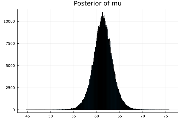
This shows that the ACTUAL PARAMETER value for mu is around 61.4

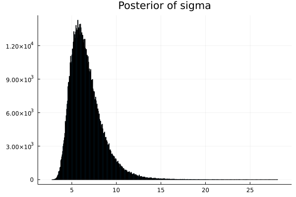
This shows that the ACTUAL PARAMETER value for mu is around 6.66

A optimized version of Metropolis Algorithm using Log function and burned in samples

Here we enhanced the algorithm by using two further optimization

Use logarithm addition instead of standard arithmetic multiplication

# The likelihood function which returns the probability,
# given a fixed mu and a fixed sigma, of the sequence of datapoints
function likelihood(data::Vector,mu::Real,sigma::Real)
    numofdatapoints = length(data)
    result=1.0
    for k = 1:numofdatapoints
        result *= pdf(Normal(mu, sigma),data[k])
    end
    return result
end

Because we are doing lots and lots and lots of multiplication, even Float64 can run out of room. Therefore most MCMC programs uses Logarithm and this ensures that Float64 will not hit its limitation.

So we do

# The likelihood function which returns the probability,
# given a fixed mu and a fixed sigma, of the sequence of datapoints
function loglikelihood(data::Vector,mu::Real,sigma::Real)
    numofdatapoints = length(data)
    result=0.0
    for k = 1:numofdatapoints
        result += log(  pdf(Normal(mu, sigma),data[k])  )
    end
    return result
end

Dispose of the burned_in_samples

We should get rid of the initial burned in samples because they are quite far away from the expected proper probability distribution of the parameter

# define the number of samples used in MCMC
# And create array parameter with that many elements (filled with 0.0)
burnedinsamples = 1000
n_samples = 1_000_000 + burnedinsamples

#= Lots of code =#

# Finally we must not forget to remove the burned in samples
deleteat!(p_μ,1:burnedinsamples)
deleteat!(p_σ,1:burnedinsamples)

So here is the complete source code

using Distributions
using StatsPlots

# Here are the weights of the students (in kilograms) in a classrom
# Assuming the weight of the students are generated by a biological
# process with a normal distribution with mean μ and standard dev σ
# find the posterior distribution of those two parameters
data = [ 55.8, 64.1, 61.2, 55.2, 58.0, 69.8, 53.2, 70.0, 63.3, 63.5 ]

# define our prior for μ as a normal centered on 60 ( required for MCMC )
prior_μ_distr = Distributions.Normal(60, 10)
prior_μ(p) = Distributions.pdf(prior_μ_distr,p)
μ_lb = 30       # Lower bound
μ_ub = 90       # Upper bound

# define our prior for σ as a exponential with mean of 20 ( required for MCMC )
prior_σ_distr = Distributions.Exponential(20)
prior_σ(p) = Distributions.pdf(prior_σ_distr,p)
σ_lb = 0        # Lower bound
σ_ub = 50       # Upper bound

# define the number of samples used in MCMC
# And create array parameter with that many elements (filled with 0.0)
burnedinsamples = 1000
n_samples = 1_000_000 + burnedinsamples
p_μ = zeros(n_samples)
p_σ = zeros(n_samples)

# Set the starting value to a random number between lb and ub
p_μ[1] = rand(prior_μ_distr)
while p_μ[1] < μ_lb || p_μ[1] > μ_ub
    p_μ[1] = rand(prior_μ_distr)
end

p_σ[1] = rand(prior_σ_distr)
while p_σ[1] < σ_lb || p_σ[1] > σ_ub
    p_σ[1] = rand(prior_σ_distr)
end


# The likelihood function which returns the probability,
# given a fixed mu and a fixed sigma, of the sequence of datapoints
function loglikelihood(data::Vector,mu::Real,sigma::Real)
    numofdatapoints = length(data)
    result=0.0
    for k = 1:numofdatapoints
        result += log(  pdf(Normal(mu, sigma),data[k])  )
    end
    return result
end

JumpingWidth = 0.01
for i in 2:n_samples
    # p_new has a value around the vicinity of p[i-1]
    p_μ_new = rand(  Normal( p_μ[i-1] , JumpingWidth*(μ_ub-μ_lb) )  )
    # make sure p_μ_new is between μ_lb and μ_ub
    if p_μ_new < μ_lb
        p_μ_new = μ_lb + abs( p_μ_new - μ_lb )
    elseif p_μ_new > μ_ub
        p_μ_new = μ_ub - abs( p_μ_new - μ_ub )
    end

    p_σ_new = rand(  Normal( p_σ[i-1] , JumpingWidth*(σ_ub-σ_lb) )  )
    # make sure p_σ_new is between σ_lb  and σ_ub
    if p_σ_new < σ_lb
        p_σ_new = σ_lb + abs( p_σ_new - σ_lb )
    elseif p_σ_new > σ_ub
        p_σ_new = σ_ub - abs( p_σ_new - σ_ub )
    end
    " q0 is posterior0 = likelihood0 * prior0        "
    " q1 is posterior1 = likelihood1 * prior1        "
#=
q0  is the probability for the CURRENT POSITION
q1  is the probability for the CANDIDATE for the NEW POSITION
=#
    logpriorμ0 = log(  prior_μ(p_μ[i-1])  )
    logpriorσ0 = log(  prior_σ(p_σ[i-1])  )
    logpriorμ1 = log(  prior_μ(p_μ_new)   )
    logpriorσ1 = log(  prior_σ(p_σ_new)   )

    logq0 = loglikelihood(data, p_μ[i-1], p_σ[i-1]) + logpriorμ0 + logpriorσ0
    logq1 = loglikelihood(data, p_μ_new, p_σ_new) + logpriorμ1 + logpriorσ1
    # The value of parameter[i] depends on whether the
    # log(random number) is less than logq1 - logq0
#=
If  the probability for the CANDIDATE for the NEW POSITION (q1)
    is GREATER than
the probability for the CURRENT POSITION (q0)
then jump to the NEW POSITION

Otherwise

Only jump to the CANDIDATE for the NEW POSITION if
a random number (between 0.0 and 1.0) is less than   q1/q0
=#
    if log(rand()) < logq1 - logq0    # Then jump to the NEW POSITION
        p_μ[i] = p_μ_new
        p_σ[i] = p_σ_new
    else        # Stick with the CURRENT POSITION
        p_μ[i] = p_μ[i-1]
        p_σ[i] = p_σ[i-1]
    end


end

# Finally we must not forget to remove the burned in samples
deleteat!(p_μ,1:burnedinsamples)
deleteat!(p_σ,1:burnedinsamples)

# Next we need to display the histogram of the array p
# this is the shape of the posterior produced by MCMC
histogram(p_μ,legend=false,title="Posterior of mu") |> display
histogram(p_σ,legend=false,title="Posterior of sigma") |> display

How to make this runs faster and easier to use

According to performance tricks for Julia

Any code that is performance critical should be inside a function. Code inside functions tends to run much faster than top level code, due to how Julia's compiler works.

The second problem is that each time we want to perform MCMC on a set of rawdata, we need to write the entire program again in Julia Programming Language.

A much better solution is to write it as a module and call the module to use MCMC.

So this version of MCMC is written as a module and it requires the following packages

Distributions
StatsPlots
Statistics
Printf
PrettyTables
DoubleFloats
CSV
DataFrames
Random

The best thing to do is to split up the code in two separate parts.

The SimpleMCMC module in a file called "SimpleMCMC.jl"
The main program in a file called "MCMC_example01.jl"
Put these two files in their own directory. Which in my case is the directory /Users/ssiew/juliascript/MCMC_dir on my Macbook
Add code to SimpleMCMC modules to save the graphics to the current directory. This would make it simple to have a copy of the graphs if we need to look at them at a later time.
Use the directory for our own enviroment when running julia.

Notes: vi is a program on unix/MacOS to edit a textfile

$ echo "This is the prompt on Terminal on MacOS"
$ cd /Users/ssiew/juliascript/MCMC_dir
$ vi SimpleMCMC.jl

# Filename is "SimpleMCMC.jl"
# Directory is "/Users/ssiew/juliascript/MCMC_dir"
using Pkg
Pkg.add(["Distributions","StatsPlots","Statistics",
"Printf","PrettyTables","DoubleFloats",
"CSV","DataFrames","Random"])

module SimpleMCMC
    export MetropolisHastings_MCMC
    export Gibbs_MCMC
    export describe_paramvec,describe_multiparamvec
    export find_best_param
    export vec2pdfcdf, find_invcdf, find_cdf, find_pdf
    export BayesFactorStrengthToString
    export findHPDI, ComparePost2Prior
    export CreateTrainTest

    using Distributions, StatsPlots, Statistics, Printf, PrettyTables
    using DoubleFloats, CSV, DataFrames, Random

    # Version 7
    #  v7: Add find_best_param, vec2pdfcdf, find_invcdf, find_cdf, find_pdf
    #  v6: Add Gibbs_MCMC and change module name from MHMCMC to SimpleMCMC
    #  v5: turn it into a module
    #  v4: remove prior from Parameter struct and the struct itself
    #  v3: create JumpingWidthVec, lbVec, ubVec  to improve efficiency
    #  v2: Remove q0 from the main loop to improve efficiency
    #  v1: Turn it into a version that uses pure function(s)

    struct Bin
        lb::Double64
        ub::Double64
        center::Double64
    end

    function MetropolisHastings_MCMC(data,lop::Vector{Distribution},loglikelihood;samples,burnedinsamples,JumpingWidth=0.01)
        # lop is "List Of Parameters"
        # Find the number of parameters
        numofparam = length(lop)
        # calc the n_samples
        n_samples = samples + burnedinsamples
        # Create a parameter Matrix p with n_samples rows and numofparam cols
        p = zeros(n_samples,numofparam)
        # JumpingWidthVector, lowerboundVector and upperboundbVector
        JumpingWidthVec = zeros(numofparam)
        lbVec = zeros(numofparam)
        ubVec = zeros(numofparam)
        # Create a Vector of our logprior function
        logpriorVec = Array{Function}(undef,numofparam)

        # Set the starting value to a random number between lb and ub
        for k = 1:numofparam  # for each parameter k
            # Set the starting value to a random number between lb and ub
            p[1,k] = rand(lop[k])

            # get 100 random values and find the practical max and practical min
            HundredRandValues = rand(lop[k],100)
            prac_min = minimum(HundredRandValues)
            prac_max = maximum(HundredRandValues)
            JumpingWidthVec[k] = JumpingWidth * (prac_max - prac_min)

            lbVec[k] = minimum(lop[k])
            ubVec[k] = maximum(lop[k])

            # Array of function prior(x) = pdf(distribution,x)
            logpriorVec[k] = x->logpdf(lop[k],x)
        end

        p_old = vec(p[1,:])
        q0 = loglikelihood(data,p_old...) + sum([logpriorVec[k](p_old[k]) for k = 1:numofparam ])

        # prepare the p_new array
        p_new = zeros(numofparam)
        # Main loop for MetropolisHastings MCMC
        @inbounds for i = 2:n_samples
            # p_new has a value around the vicinity of p[i-1]
            for k = 1:numofparam  # for each parameter k
                # p_new has a value around the vicinity of p[i-1]
                p_new[k] = rand(  Normal( p[i-1,k] , JumpingWidthVec[k] )  )
                # make sure p_new is between lb and ub
                if p_new[k] < lbVec[k]
                    p_new[k] = lbVec[k] + abs( p_new[k] - lbVec[k] )
                elseif p_new[k] > ubVec[k]
                    p_new[k] = ubVec[k] - abs( p_new[k] - ubVec[k] )
                end
            end

            # Calc the two posterior
            " q0 is posterior0 = likelihood0 * prior0        "
            " q1 is posterior1 = likelihood1 * prior1        "
            q1 = loglikelihood(data,p_new...) + sum([logpriorVec[k](p_new[k]) for k = 1:numofparam ])
            # The value of p[i] depends on whether the
            # random number is less than q1/q0
            p[i,:] .= log(rand()) < q1-q0 ? (q0=q1; p_old=p_new[:]) : p_old
        end
        # Finally we must not forget to remove the burned in samples
        return p[(burnedinsamples+1):end,:]
    end

    function Gibbs_MCMC(data,lop::Vector{Distribution},loglikelihood;samples,burnedinsamples)
        # lop is "List Of Parameters"
        # Find the number of parameters
        numofparam = length(lop)
        # calc the n_samples
        n_samples = samples + burnedinsamples
        # Create a parameter Matrix p with n_samples rows and numofparam cols
        p = zeros(n_samples,numofparam)
        # Number of holes to drill
        numofdrillholes = 1001
        drillhole = Array{Float64}(undef,numofdrillholes)
        mycdf = Array{Double64}(undef,numofdrillholes+1)
        # prepare the vectors: startposvec stopposvec chunksizevec
        startposvec = zeros(numofparam)
        stopposvec = zeros(numofparam)
        chunksizevec = zeros(numofparam)

        # Set the starting value to a random number between lb and ub
        for k = 1:numofparam  # for each parameter k
            # Set the starting value to a random number between lb and ub
            p[1,k] = rand(lop[k])

            # get 400 random values and find the practical max and practical min
            FourHundredRandValues = rand(lop[k],400)
            startposvec[k] = minimum(FourHundredRandValues)
            stopposvec[k]  = maximum(FourHundredRandValues)
            chunksizevec[k] = (stopposvec[k]-startposvec[k])/(numofdrillholes-1)
        end

        # Main loop for Gibbs MCMC
        @inbounds for i = 2:n_samples
            # prepare the p_new vector
            p_new = vec(p[i-1,:])
            # Select a new value for each parameter of p_new
            for k = 1:numofparam  # for each parameter k
                # Calculate chunk size
                startpos,stoppos,chunksize = startposvec[k],stopposvec[k],chunksizevec[k]
                mycdf[1] = Double64(0.0)
                # Start drilling the drill holes for parameter k
                for n = 1:numofdrillholes
                    p_new[k] = startpos + (n-1) * chunksize
                    drillhole[n] = exp(  loglikelihood(data,p_new...)  )
                    mycdf[n+1] = mycdf[n] + drillhole[n]
                end
                mycdf /= mycdf[end]
                # Now we perform an inverse CDF sampling
                x = 0.0
                while x == 0.0
                    x = rand()  # Make sure x is not zero
                end
                counter = 2
                while !(mycdf[counter-1] < x <= mycdf[counter])
                    counter += 1
                end
                counter -= 1
                # now find the kth parameter value
                pos = startpos + (counter-1) * chunksize
                # This is the value we are going to jump to
                p_new[k] = pos
                p[i,k] = pos
            end
        end
        # Finally we must not forget to remove the burned in samples
        return p[(burnedinsamples+1):end,:]
    end

    function describe_paramvec(name,namestr,v::Vector)
        m,s,v_sorted = mean(v),std(v),sort(v)
        pc5 = v_sorted[Int64(round(0.055*length(v_sorted)))]
        pc94 = v_sorted[Int64(round(0.945*length(v_sorted)))]
        println(
            "Parameter $(name)   mean ",@sprintf("%6.3f",round(m,sigdigits=3)),
            "   sd ",@sprintf("%6.3f",round(s,sigdigits=3)),
            "   5.5% ",@sprintf("%6.3f",round(pc5,sigdigits=3)),
            "   94.5% ",@sprintf("%6.3f",round(pc94,sigdigits=3))
        )
        histogram(v,legend=false,title="Posterior of $(namestr)") |> display
        return (m,s,pc5,pc94)
    end

    function describe_multiparamvec(multi::Vector;savegraph=false)
        # name,namestr,v::Vector
        numofparams = length(multi)
        table = Array{Any}(undef,numofparams,5)
        for i = 1:numofparams
            v = multi[i][3]
            m,s,v_sorted = mean(v),std(v),sort(v)
            pc5 = v_sorted[Int64(round(0.055*length(v_sorted)))]
            pc94 = v_sorted[Int64(round(0.945*length(v_sorted)))]
            table[i,1]=multi[i][1]
            table[i,2],table[i,3],table[i,4],table[i,5]=m,s,pc5,pc94
            histogram(v,legend=false,title="Posterior of $(multi[i][2])") |> display
            # Save the graphics to the current directory
            if savegraph
                savefig("Posterior of $(multi[i][2]).png")
            end
        end
        pretty_table(table;
            header = tuple(["Parameter","Mean","Stddev","5.5%","94.5%"]),
            alignment=:l,
            #formatter=Dict(0 => (v,i) -> typeof(v) <: Number ? round(v,sigdigits=3) : v )
            formatters=((v,i,j) -> typeof(v) <: Number ? round(v,sigdigits=3) : v,)
        )
        return table
    end

    function find_best_param(data,param_mat,loglikelihood)
        bestpos = 0
        bestscore = -Inf
        for k = 1:size(param_mat,1)
            currscore = loglikelihood(data,param_mat[k,:]...)
            if currscore > bestscore
                bestscore = currscore
                bestpos = k
            end
        end
        return (bestpos,bestscore)
    end

    function vec2pdfcdf(vec::Vector,nbins::Int64=20)
        vec_sorted = sort(vec)
        len = length(vec)
        pc0001_pos = Int64(round(len * 0.0001,RoundDown))
        pc0001_pos = pc0001_pos > 0 ? pc0001_pos : 1
        pc9999_pos = Int64(round(len * 0.9999,RoundDown))
        pc9999_pos = pc9999_pos < len ? pc9999_pos : len

        chunksize = (Double64(vec_sorted[pc9999_pos]) -
                     Double64(vec_sorted[pc0001_pos])) / Double64(nbins-2)
        bins = Vector{Bin}(undef,nbins)
        binscount = Int64[ 0 for k = 1:nbins ]
        bins[1]   = Bin(Double64(vec_sorted[pc0001_pos]) - chunksize,
                        Double64(vec_sorted[pc0001_pos]),
                        Double64(vec_sorted[pc0001_pos]) - (chunksize/df64"2.0"))
        bins[end] = Bin(Double64(vec_sorted[pc9999_pos]),
                        Double64(vec_sorted[pc9999_pos]) + chunksize,
                        Double64(vec_sorted[pc9999_pos]) + (chunksize/df64"2.0"))
        # Create and specify each bin
        for k = 2:nbins-1
            bins[k] = Bin(bins[1].ub+(k-2)*chunksize,
                          bins[1].ub+(k-1)*chunksize,
                          bins[1].ub+(k-1.5)*chunksize)
        end
        # Now perform the histogram function
        for n = 1:len
            ((vec[n] < bins[1].lb) || (vec[n] >= bins[end].ub)) && continue
            k=1
            while !(bins[k].lb <= vec[n] < bins[k].ub)
                k +=1
            end
            binscount[k] += 1
        end
        binscount_total = sum(binscount)
        # Now perform normalization
        pdfvalue = Float64[ Float64(binscount[k]/binscount_total) for k = 1:nbins ]
        # println("Sum of binsvalue is ",sum(binsvalue))
        centervec = Float64[ Float64(bins[k].center) for k = 1:nbins ]
        # Now create cdf
        cdfcount = Array{Int64}(undef,nbins)
        cdfcount[1] = binscount[1]
        for k = 2:nbins
            cdfcount[k] = cdfcount[k-1] + binscount[k]
        end
        cdfvalue = Float64[ Float64(cdfcount[k]/binscount_total) for k = 1:nbins ]
        return (centervec,pdfvalue,cdfvalue)
    end

    function find_invcdf(gridvec,cdfvec,x)
        if x < cdfvec[1]
            return gridvec[1]
        end
        counter = 2
        while !(cdfvec[counter-1] < x <= cdfvec[counter])
            counter += 1
        end
        return gridvec[counter]
    end

    function find_cdf(gridvec,cdfvec,x)
        len = length(gridvec)
        width = gridvec[2] - gridvec[1]
        # estimate counter
        startpos = gridvec[1] - 1.5 * width
        k = Int64(round((x - startpos)/width,RoundDown))
        if k < 1
            return 0.0
        elseif  k > len
            return 1.0
        else
            return cdfvec[k]
        end
    end

    function find_pdf(gridvec,pdfvec,x)
        len = length(gridvec)
        width = gridvec[2] - gridvec[1]
        # estimate counter
        startpos = gridvec[1] - 1.5 * width
        k = Int64(round((x - startpos)/width,RoundDown))
        if k < 1 || k > len
            return 0.0
        else
            return pdfvec[k]
        end
    end

    function BayesFactorStrengthToString(x)
        if 10.0^0.0 <= x < 10.0^0.5
            return "Barely worth mentioning"
        elseif 10.0^0.5 <= x < 10.0^1.0
            return "Substantial"
        elseif 10.0^1.0 <= x < 10.0^1.5
            return "Strong"
        elseif 10.0^1.5 <= x < 10.0^2.0
            return "Very Strong"
        elseif 10.0^2.0 <= x
            return "Decisive"
        else
            return "AGAINST at " * BayesFactorStrength(1.0/x)
        end
    end

    # Now we create the function findHPDI()
    function findHPDI(grid::Vector,pdf::Vector,mass,depth)
        len_grid,len_pdf = length(grid),length(pdf)
        @assert len_grid == len_pdf "Grid vector and pdf vector does not have the same length"
        result = findHPDI_coarsegrain(depth,mass,1,len_pdf,pdf)
        # We have done the course grain, so now we need to
        # do the fine grain adjustment
        while true
            # Create a list of candidates
            candidates = []
            for startadj = -10:10
                for stopadj = -10:10
                    cand = (  max(result[1]+startadj,1),
                              min(result[2]+stopadj,len_pdf)
                           )
                    push!(candidates,cand)
                end
            end
            # We need to evaluate the candidates by one criterion
            # The criterion is mininum mass
            eligible = []
            for candidate in candidates
                candidate_mass = sum(pdf[candidate[1]:candidate[2]])
                candidate_width = candidate[2]-candidate[1]
                if  candidate_mass >= mass && candidate_width > 0
                    candidate_density = candidate_mass / candidate_width
                    push!(eligible,[candidate_density,candidate])
                    #= println("FG: candidate ",candidate," has mass ",
                    candidate_mass,
                    " and density ",candidate_density)
                    =#
                end
            end
            sort!(eligible)
            # println(eligible)
            # Now extract the best candidate
            best = eligible[end]
            best_density = best[1]
            best_candidate = best[2]
            best_mass = sum(pdf[best_candidate[1]:best_candidate[2]])
            #= println("FG: Best candidate ",best_candidate,
            "has mass ",best_mass,
            " has density ",best_density)
            =#
            # Now call itself recursively
            if best_candidate[1] == result[1] && best_candidate[2] == result[2]
                # There is no point recursing down any further as
                # we reached the limit of recursion
                return result
            else
                # Subtract the depth level and recurse down further
                result = best_candidate
            end
        end
    end

    function findHPDI_coarsegrain(depth::Integer,mass,start,stop,pdf)
        @assert start <= stop "start is greater than stop"
        if depth < 1 || stop == start || stop == start + 1
            return (start,stop)
        end
        len = stop - start
        chunk = len ÷ 3
        # Handle special case where chunk is zero
        if chunk == 0
            # This is the limit of Coarse Grain algorithmn
            return (start,stop)
        end
        # There are four points
        point1 = start
        point2 = start + chunk
        point3 = start + 2 * chunk
        point4 = stop
        # From these four points,
        # we can produce 5 candidates
        candidate1 = (point1,point2)
        candidate2 = (point1,point3)
        candidate3 = (point2,point3)
        candidate4 = (point2,point4)
        candidate5 = (point3,point4)
        candidate6 = (point1,point4)
        # Create a list of candidates
        candidates = [ candidate1, candidate2, candidate3, candidate4, candidate5, candidate6 ]
        # We need to evaluate the candidates by one criterion
        # The criterion is mininum mass
        eligible = []
        for candidate in candidates
            candidate_mass = sum(pdf[candidate[1]:candidate[2]])
            candidate_width = candidate[2]-candidate[1]
            candidate_density = candidate_mass / candidate_width
            if  candidate_mass >= mass
                push!(eligible,[candidate_density,candidate])
                #= println("candidate ",candidate," has mass ",
                candidate_mass,
                " and density ",candidate_density)
                =#
            end
        end
        sort!(eligible)
        # println(eligible)
        # Now extract the best candidate
        best = eligible[end]
        best_density = best[1]
        best_candidate = best[2]
        #= println("Best candidate ",best_candidate,
        " has density ",best_density)
        =#
        # Now call itself recursively
        if best_candidate[1] == start && best_candidate[2] == stop
            # There is no point recursing down any further as
            # we reached the limit of recursion
            return (start,stop)
        else
            # Subtract the depth level and recurse down further
            return findHPDI_coarsegrain(depth-1,mass,best_candidate[1],best_candidate[2],pdf)
        end
    end

    function ComparePost2Prior(prior,vec,nbins=1001;kwargs...)
        lb = minimum(prior)
        ub = maximum(prior)
        if lb == -Inf || ub == Inf
            FourHundredRandValues = rand(prior,400)
            lb = lb == -Inf ? minimum(FourHundredRandValues) : lb
            ub = ub ==  Inf ? maximum(FourHundredRandValues) : ub
        end
        prior_range = range(lb,length=1001,stop=ub)
        (centervec,pdfvalue,cdfvalue) = vec2pdfcdf(vec,nbins)
        prior_vec = [ pdf(prior,x) for x in prior_range ]
        pdf_vec = [ find_pdf(centervec,pdfvalue,x) for x in prior_range ]
        scaling_factor = sum(prior_vec)/sum(pdf_vec)
        pdf_vec = pdf_vec * scaling_factor
        plot(prior_range,[prior_vec,pdf_vec],
            xlimit=(lb,ub),legend=false;kwargs...
        ) |> display
    end

    function CreateTrainTest(df::DataFrame,prop=0.5,randomseed=1234)
        df_training = similar(df,0)
        df_testing  = similar(df,0)

        # Now split the df into df_training and df_testing
        df_size = size(df,1)
        training_proportion = prop
        trainingsize = round(df_size*training_proportion)

        # Create a random permutaion vector
        randvec = randperm!(MersenneTwister(randomseed),
                            Vector{Int64}(undef,df_size))

        for k in axes(df)[1]
            push!(  k ≤ trainingsize ?
                    df_training : df_testing ,
                    df[randvec[k],:]
            )
        end
        return (df_training,df_testing)
    end

end
#= End of module SimpleMCMC =#

$ echo "This is the prompt on Terminal on MacOS"
$ cd /Users/ssiew/juliascript/MCMC_dir
$ vi MCMC_example01.jl

# Filename is "MCMC_example01.jl"
# Directory is "/Users/ssiew/juliascript/MCMC_dir"

# include the source code for the SimpleMCMC module
include("/Users/ssiew/juliascript/MCMC_dir/SimpleMCMC.jl")

using Distributions, StatsPlots, Statistics
using .SimpleMCMC

function MCMC_example()

    # Here are the weights of the students (in kilograms) in a classrom
    # Assuming the weight of the students are generated by a biological
    # process with a normal distribution with mean μ and standard dev σ
    # find the posterior distribution of those two parameters
    data = [ 55.8, 64.1, 61.2, 55.2, 58.0, 69.8, 53.2, 70.0, 63.3, 63.5 ]

    # define our prior for μ as a normal centered on 60 ( required for MCMC )
    μ = Normal(60, 10)
    # define our prior for σ as a exponential with mean of 20 ( required for MCMC )
    σ = Exponential(20)

    # Put all our parameters into a list
    ListOfParams = Distribution[μ,σ]

    # The loglikelihood function which returns the log(probability),
    # given a fixed mu and a fixed sigma, of the sequence of datapoints
    function loglikelihood(data::Vector,mu,sigma)
        numofdatapoints = length(data)
        result=0.0
        for k = 1:numofdatapoints
            result += logpdf(Normal(mu,sigma),data[k])
        end
        return result
    end

    p = MetropolisHastings_MCMC(
            data,
            ListOfParams,
            loglikelihood,
            samples=1_000_000,
            burnedinsamples=1000
    )

    # Next we need to display the histogram of the column p[:,1]
    # this is the shape of the posterior produced by MCMC
    vec_μ=vec(p[:,1])  # Convert a Matrix column into a 1-D Vector
    vec_σ=vec(p[:,2])  # Convert a Matrix column into a 1-D Vector
    #describe_paramvec("μ","mu",vec_μ)
    #describe_paramvec("σ","sigma",vec_σ)
    describe_multiparamvec([("μ","mu",vec_μ),("σ","sigma",vec_σ)])
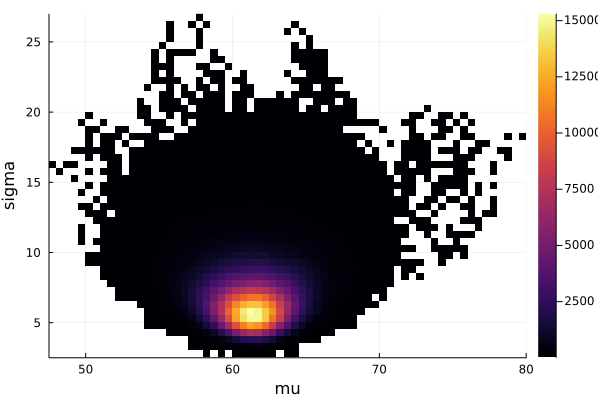
    histogram2d(vec_μ,vec_σ,nbins=100,xlabel="mu",ylabel="sigma") |> display
    # save the graphics to the current directory
    savefig("histogram2D_mu_sigma.png")
end

# We call the main function to kick off the example
MCMC_example()

Now we can call Julia on the terminal to run the script

$ echo "This is the prompt on Terminal on MacOS"
$ cd /Users/ssiew/juliascript/MCMC_dir
$ julia --project=. MCMC_example01.jl

Starting Julia...
               _
   _       _ _(_)_     |  Documentation: https://docs.julialang.org
  (_)     | (_) (_)    |
   _ _   _| |_  __ _   |  Type "?" for help, "]?" for Pkg help.
  | | | | | | |/ _  |  |
  | | |_| | | | (_| |  |  Version 1.8.5 (2023-01-08)
 _/ |\__'_|_|_|\__'_|  |  Official https://julialang.org/ release
|__/                   |
[ Info: Precompiling SimpleMCMC [top-level]
┌───────────┬──────┬────────┬──────┬───────┐
│ Parameter │ Mean │ Stddev │ 5.5% │ 94.5% │
├───────────┼──────┼────────┼──────┼───────┤
│ μ         │ 61.4 │ 2.09   │ 58.1 │ 64.6  │
│ σ         │ 6.66 │ 1.85   │ 4.44 │ 9.89  │
└───────────┴──────┴────────┴──────┴───────┘

What can MCMC do that ordinary high school statistics can't do?

So far, you have been underwhelm by the MCMC tool. We got a bunch of student weights and found the mean and standard deviation of the students. Big deal! Ordinary high school statistics can do that!

Why go through so much complex programming just to find the mean and standard deviation? It really really felt much ado about nothing. Please show us something that MCMC can do and high school statistics CANNOT DO.

Okay. Consider this problem. There are 100 students in a class. 55% of the students are male and 45% of the students are female. The teacher measured the heights of the students in metres. The teacher DID NOT record down the name or the gender of each student.

Your mission, if you can even do it, is to find the mean and standard deviation of

The male students
The female students

Now this really is mission impossible as the male students and female students are mixed together. You cannot simply tell from a height if the student is male or if the student is female and yet you have to "somehow" seperate them into two gender and then calculate their gender mean and gender standard deviation.

This is truely something that high school statistics cannot do.

Generate 100 datapoints

First thing first, we need to generate 100 datapoints to represent the height of the students. We also need to make sure that we get the same datapoints each time. To do so, we use StableRNGs which guarranty that we get the same random numbers everytime (even if the Julia version changes).

In the code below, we use the following ACTUAL PARAMETERS

μm_actual = 1.76 (male mean)
σm_actual = 0.0635 (male std dev)
μf_actual = 1.62 (female mean)
σf_actual = 0.0559 (female std dev)

These will be the numbers that we can trying to estimate using MCMC

using StableRNGs,Distributions

function generatedata(;numofdatum = 100)
    rng = StableRNG(12345)
    data = zeros(numofdatum)
    # 55% male with 1.76 m and std dev of 0.0635
    for k = 1:Int64(55//100*numofdatum)
        data[k] = rand(rng,Normal(1.76,0.0635))
    end
    # 45% female with 1.62 m and std dev of 0.0559
    for k = (1+Int64(55//100*numofdatum)):numofdatum
        data[k] = rand(rng,Normal(1.62,0.0559))
    end
    return round.(data,digits=2)
end

data = generatedata()

Error Score

As we know what the Actual Parameter values are, we can compute how wrong our estimates are.

We defined a function called errorscore to compute the error score value where the large the error score is, the more wrong the estimated values are when compare to the actual values.

First attempt

# Filename is "bothgender01.jl"
# Directory is "/Users/ssiew/juliascript/MCMC_dir"
include("/Users/ssiew/juliascript/MCMC_dir/SimpleMCMC.jl")

using Distributions, StatsPlots, Statistics
using .SimpleMCMC
using StableRNGs,Distributions

const μm_actual = 1.76
const σm_actual = 0.0635
const μf_actual = 1.62
const σf_actual = 0.0559

ActualParameters = [μm_actual,σm_actual,μf_actual,σf_actual]

function generatedata(;numofdatum = 100)
    rng = StableRNG(12345)
    data = zeros(numofdatum)
    # 55% male with 1.76 m and std dev of 0.0635
    for k = 1:Int64(55//100*numofdatum)
        data[k] = rand(rng,Normal(μm_actual,σm_actual))
    end
    # 45% female with 1.62 m and std dev of 0.0559
    for k = (1+Int64(55//100*numofdatum)):numofdatum
        data[k] = rand(rng,Normal(μf_actual,σf_actual))
    end
    return round.(data,digits=2)
end

# Generate a numeric score so that we can compare how MCMC is performing
function errorscore(actual_parameter, estimated_parameter, scalingfactor, weighting)
    local temp
    temp = actual_parameter .- estimated_parameter
    temp = temp ./ scalingfactor
    temp = temp .^ 2
    temp = temp .* weighting
    return round(sum(temp),sigdigits=3)
end

function MCMC_example()

    data = generatedata()

    μm = Normal(1.6, 0.5)
    σm = Uniform(0.0,1.0)
    μf = Normal(1.6, 0.5)
    σf = Uniform(0.0,1.0)

    # Put all our parameters into a list
    ListOfParams = Distribution[μm,σm,μf,σf]

    # The loglikelihood function which returns the log(probability),
    # given a fixed mu and a fixed sigma, of the sequence of datapoints
    function loglikelihood(data::Vector,μm,σm,μf,σf)
        numofdatapoints = length(data)
        result=0.0
        @inbounds for k = 1:numofdatapoints
            mmm = 0.55*pdf(Normal(μm,σm),data[k])
            fff = 0.45*pdf(Normal(μf,σf),data[k])
            result += log(   mmm + fff   )
        end
        return result
    end

    p = MetropolisHastings_MCMC(
            data,
            ListOfParams,
            loglikelihood,
            samples=1_000_000,
            burnedinsamples=1000
    )

    # Next we need to display the histogram of the column p[:,1]
    # this is the shape of the posterior produced by MCMC
    vec_μm=vec(p[:,1])  # Convert a Matrix column into a 1-D Vector
    vec_σm=vec(p[:,2])  # Convert a Matrix column into a 1-D Vector
    vec_μf=vec(p[:,3])  # Convert a Matrix column into a 1-D Vector
    vec_σf=vec(p[:,4])  # Convert a Matrix column into a 1-D Vector
    #describe_paramvec("μ","mu",vec_μ)
    #describe_paramvec("σ","sigma",vec_σ)
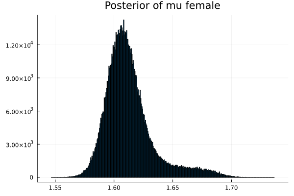
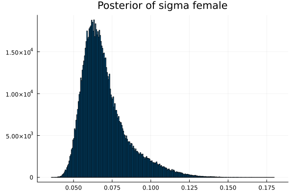
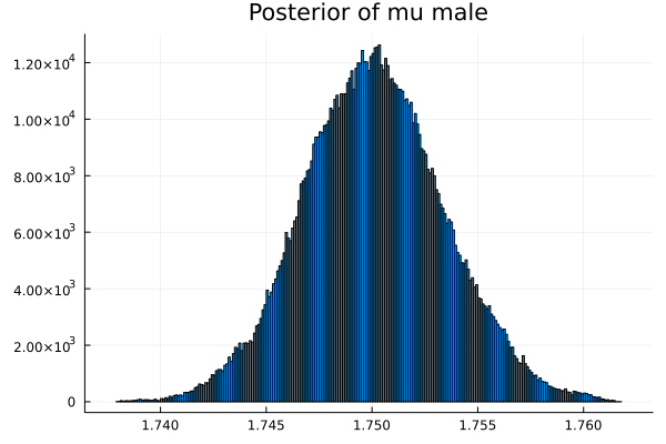
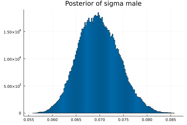
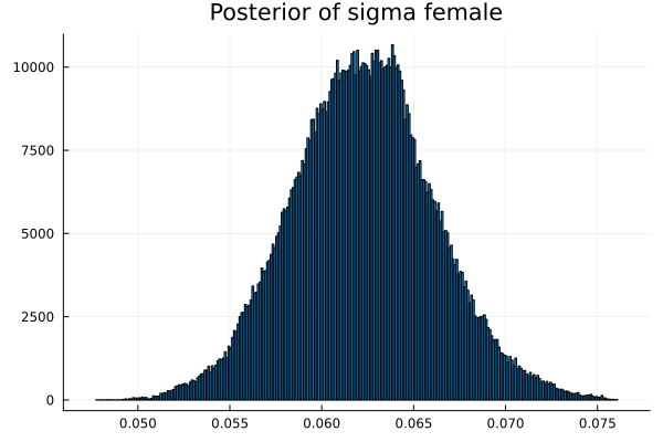
    t = describe_multiparamvec([("μm","mu male",vec_μm),
                            ("σm","sigma male",vec_σm),
                            ("μf","mu female",vec_μf),
                            ("σf","sigma female",vec_σf)
                            ],savegraph=true)
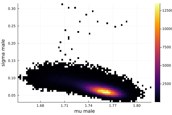
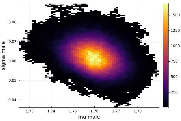
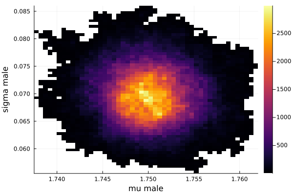
    histogram2d(vec_μm,vec_σm,nbins=100,xlabel="mu male",ylabel="sigma male") |> display
    savefig("histogram2D_mu_male_sigma_male.png")
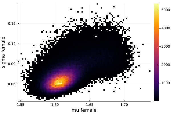
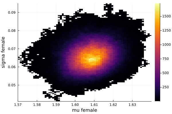
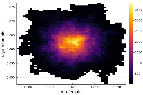
    histogram2d(vec_μf,vec_σf,nbins=100,xlabel="mu female",ylabel="sigma female") |> display
    savefig("histogram2D_mu_female_sigma_female.png")
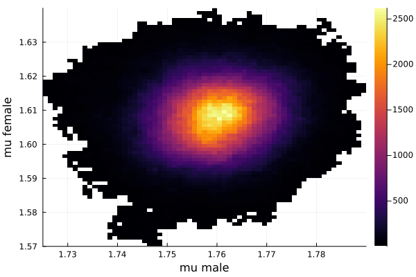
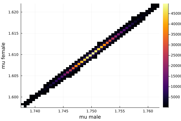
    histogram2d(vec_μm,vec_μf,nbins=100,xlabel="mu male",ylabel="mu female") |> display
    savefig("histogram2D_mu_male_mu_female.png")
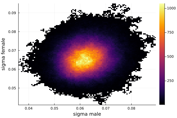
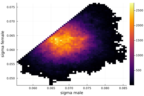
    histogram2d(vec_σm,vec_σf,nbins=100,xlabel="sigma male",ylabel="sigma female") |> display
    savefig("histogram2D_sigma_male_sigma_female.png")

    estimated = round.(t[:,2],sigdigits=3)

    println("error score is ",
        errorscore(
        ActualParameters,
        estimated,
        [0.01,0.01,0.01,0.01],
        [1/4,1/4,1/4,1/4]
        )
    )
end

# We call the main function to kick off the example
MCMC_example()

Prior

Now we need to explain our prior.

We knows most humans are around 1.6 metres tall and their standard deviation is a lot less than 0.5 metres. So we set the prior for mean for height to be:

Normal(1.6,0.5) for both males and females.

We set the prior for standard deviation for height to be

Uniform(0.0,1.0)

Because it has to be greater than zero but less than 1 metre

loglikelihood function

The pdf (probability density function) of the distribution of height for the students is the weighted combination of the pdf distribution of both the genders of the students.

0.55 * pdf(male height distribution) + 0.45 * pdf(female height distribution)

function loglikelihood(data::Vector,μm,σm,μf,σf)
    numofdatapoints = length(data)
    result=0.0
    @inbounds for k = 1:numofdatapoints
        mmm = 0.55*pdf(Normal(μm,σm),data[k])
        fff = 0.45*pdf(Normal(μf,σf),data[k])
        result += log(   mmm + fff   )
    end
    return result
end

results

So here are the results

$ echo "This is the prompt on Terminal on MacOS"
$ cd /Users/ssiew/juliascript/MCMC_dir
$ julia --project=. bothgender01.jl

Starting Julia...
               _
   _       _ _(_)_     |  Documentation: https://docs.julialang.org
  (_)     | (_) (_)    |
   _ _   _| |_  __ _   |  Type "?" for help, "]?" for Pkg help.
  | | | | | | |/ _  |  |
  | | |_| | | | (_| |  |  Version 1.8.5 (2023-01-08)
 _/ |\__'_|_|_|\__'_|  |  Official https://julialang.org/ release
|__/                   |
[ Info: Precompiling SimpleMCMC [top-level]
┌───────────┬────────┬────────┬────────┬────────┐
│ Parameter │ Mean   │ Stddev │ 5.5%   │ 94.5%  │
├───────────┼────────┼────────┼────────┼────────┤
│ μm        │ 1.67   │ 0.0649 │ 1.6    │ 1.77   │
│ σm        │ 0.071  │ 0.0136 │ 0.0525 │ 0.0957 │
│ μf        │ 1.71   │ 0.0781 │ 1.59   │ 1.79   │
│ σf        │ 0.0614 │ 0.016  │ 0.0419 │ 0.0921 │
└───────────┴────────┴────────┴────────┴────────┘
error score is 45.5

Analysis of First attempt

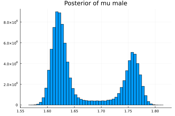
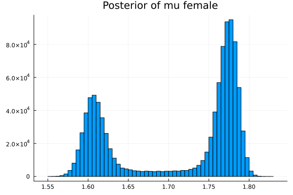
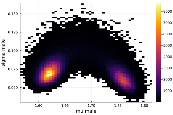
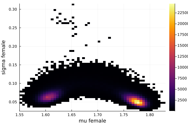
The first thing we noticed about results is that MCMC thinks that the mean of the male height has two peaks. They are 1.77 m and 1.62 m.

It also thinks that the mean of the female height has two peaks. They are also 1.77 m and 1.62 m.

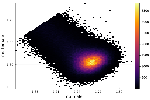
This woukld be clearer when we look at the 2D histogram of “mu male” vs “mu female”. It shows two distinct peaks.

one peak is (mu male=1.62,mu female=1.77)
the other peak is (mu male=1.77,mu female=1.66)

After thinking about it, it became clear that these are the two possibilities that will generate the distribution of the overall student heights. The MCMC does NOT know which of the two possibilities is responsible for the datapoints.

Where as we humans know (through our common sense) that the average height of males is higher than the average height of females.

So what we need to do is to inform MCMC of the fact that mean of male height is ALWAYS higher than the mean of the female height.

Second attempt

Let's alter the source code to let the MCMC know that mean of males are higher than mean of females.

We do this by changing the loglikelihood function to reduce each component of the result (per datapoint) by -1.0 if μf > μm.

we use (the reverse logic)

(μm > μf ? 0.0 : -1.0)

# Filename is "bothgender02.jl"
# Directory is "/Users/ssiew/juliascript/MCMC_dir"
include("/Users/ssiew/juliascript/MCMC_dir/SimpleMCMC.jl")

using Distributions, StatsPlots, Statistics
using .SimpleMCMC
using StableRNGs,Distributions

const μm_actual = 1.76
const σm_actual = 0.0635
const μf_actual = 1.62
const σf_actual = 0.0559

ActualParameters = [μm_actual,σm_actual,μf_actual,σf_actual]

function generatedata(;numofdatum = 100)
    rng = StableRNG(12345)
    data = zeros(numofdatum)
    # 55% male with 1.76 m and std dev of 0.0635
    for k = 1:Int64(55//100*numofdatum)
        data[k] = rand(rng,Normal(μm_actual,σm_actual))
    end
    # 45% female with 1.62 m and std dev of 0.0559
    for k = (1+Int64(55//100*numofdatum)):numofdatum
        data[k] = rand(rng,Normal(μf_actual,σf_actual))
    end
    return round.(data,digits=2)
end

# Generate a numeric score so that we can compare how MCMC is performing
function errorscore(actual_parameter, estimated_parameter, scalingfactor, weighting)
    local temp
    temp = actual_parameter .- estimated_parameter
    temp = temp ./ scalingfactor
    temp = temp .^ 2
    temp = temp .* weighting
    return round(sum(temp),sigdigits=3)
end

function MCMC_example()

    data = generatedata()

    μm = Normal(1.6, 0.5)
    σm = Uniform(0.0,1.0)
    μf = Normal(1.6, 0.5)
    σf = Uniform(0.0,1.0)

    # Put all our parameters into a list
    ListOfParams = Distribution[μm,σm,μf,σf]

    # The loglikelihood function which returns the log(probability),
    # given a fixed mu and a fixed sigma, of the sequence of datapoints
    function loglikelihood(data::Vector,μm,σm,μf,σf)
        numofdatapoints = length(data)
        result=0.0
        @inbounds for k = 1:numofdatapoints
            mmm = 0.55*pdf(Normal(μm,σm),data[k])
            fff = 0.45*pdf(Normal(μf,σf),data[k])
            result += (  log(   mmm + fff   )     +
                         (μm > μf ? 0.0 : -1.0)
                      )
        end
        return result
    end

    p = MetropolisHastings_MCMC(
            data,
            ListOfParams,
            loglikelihood,
            samples=1_000_000,
            burnedinsamples=1000
    )

    # Next we need to display the histogram of the column p[:,1]
    # this is the shape of the posterior produced by MCMC
    vec_μm=vec(p[:,1])  # Convert a Matrix column into a 1-D Vector
    vec_σm=vec(p[:,2])  # Convert a Matrix column into a 1-D Vector
    vec_μf=vec(p[:,3])  # Convert a Matrix column into a 1-D Vector
    vec_σf=vec(p[:,4])  # Convert a Matrix column into a 1-D Vector
    #describe_paramvec("μ","mu",vec_μ)
    #describe_paramvec("σ","sigma",vec_σ)
    t = describe_multiparamvec([("μm","mu male",vec_μm),
                            ("σm","sigma male",vec_σm),
                            ("μf","mu female",vec_μf),
                            ("σf","sigma female",vec_σf)
                            ],savegraph=true)
    histogram2d(vec_μm,vec_σm,nbins=100,xlabel="mu male",ylabel="sigma male") |> display
    savefig("histogram2D_mu_male_sigma_male.png")
    histogram2d(vec_μf,vec_σf,nbins=100,xlabel="mu female",ylabel="sigma female") |> display
    savefig("histogram2D_mu_female_sigma_female.png")
    histogram2d(vec_μm,vec_μf,nbins=100,xlabel="mu male",ylabel="mu female") |> display
    savefig("histogram2D_mu_male_mu_female.png")
    histogram2d(vec_σm,vec_σf,nbins=100,xlabel="sigma male",ylabel="sigma female") |> display
    savefig("histogram2D_sigma_male_sigma_female.png")

    estimated = round.(t[:,2],sigdigits=3)

    println("error score is ",
        errorscore(
        ActualParameters,
        estimated,
        [0.01,0.01,0.01,0.01],
        [1/4,1/4,1/4,1/4]
        )
    )
end

# We call the main function to kick off the example
MCMC_example()

results Second Attempt

So here are the results

$ echo "This is the prompt on Terminal on MacOS"
$ cd /Users/ssiew/juliascript/MCMC_dir
$ julia --project=. bothgender02.jl

Starting Julia...
               _
   _       _ _(_)_     |  Documentation: https://docs.julialang.org
  (_)     | (_) (_)    |
   _ _   _| |_  __ _   |  Type "?" for help, "]?" for Pkg help.
  | | | | | | |/ _  |  |
  | | |_| | | | (_| |  |  Version 1.8.5 (2023-01-08)
 _/ |\__'_|_|_|\__'_|  |  Official https://julialang.org/ release
|__/                   |
┌───────────┬────────┬────────┬────────┬────────┐
│ Parameter │ Mean   │ Stddev │ 5.5%   │ 94.5%  │
├───────────┼────────┼────────┼────────┼────────┤
│ μm        │ 1.75   │ 0.0195 │ 1.71   │ 1.78   │
│ σm        │ 0.0664 │ 0.0142 │ 0.0487 │ 0.0938 │
│ μf        │ 1.61   │ 0.0209 │ 1.59   │ 1.66   │
│ σf        │ 0.0702 │ 0.0151 │ 0.0524 │ 0.1    │
└───────────┴────────┴────────┴────────┴────────┘
error score is 1.03

Analysis of Second attempt

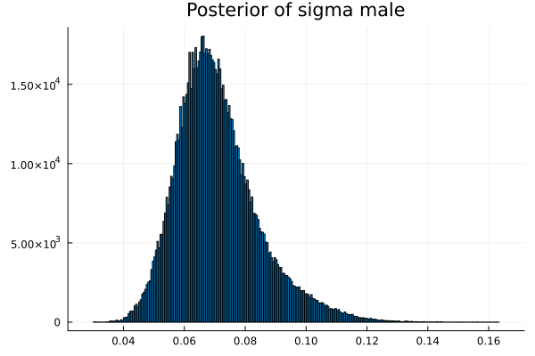
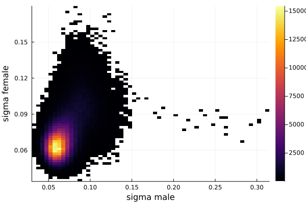
Now the results are so much better than the first attempt. For one, we got a single peak for the mean height for males and a single peak for the mean height for females.

And the 2D histogram of “mu male” vs “mu female” also shows a single peak. This is very good news indeed!

Fit booster using Turbo Cycle

Is there any other method where the error score can be further reduced? Well, we could use the turbo mode.

How Turbo Cycle works

In a car, the basic concept of a Turbo Charger is to use the ultra high pressure of the exhaust gas to power an air compressor in order to compress the intake air to an higher air pressure before it enters an engine.

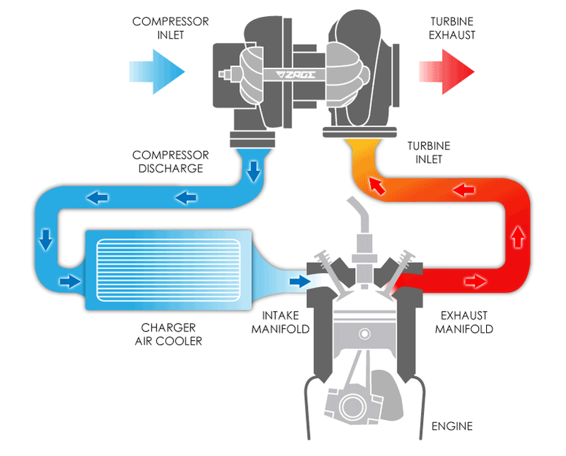
But why do turbo chargers work? The secret is that the amount of energy liberated by the internal combustion engine is dependant on two things.

amount of fuel molecules
amount of oxygen molecules

While we have no problems with putting in as much fuel as we want. The only way to increase the amount of oxygen molecules is to increase the air pressure of the intake air using an air compressor. Otherwise we are LIMITED by

18% oxygen gas in the atmosphere (the rest is mostly Nitrogen gas)
1.0 standard air pressure in the atmosphere

Back to explaination, we use use the POWER OF THE EXHAUST to increase the QUALITY OF THE AIR INTAKE. or you can say "We use the HIGH PRESSURE of the exhaust gas to further increase the air pressure of the air intake."

With MCMC, we have the exactly same issue.

The PRIOR of the input to MCMC is basically very LOW QUALITY.
The output of the MCMC is HIGHER QUALITY POSTERIOR

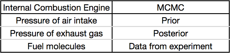
The idea is to use the "HIGHER QUALITY POSTERIOR" as the PRIOR for the next cycle of the MCMC input.

Limitation of Turbo Cycle

The limiting factor of course is the Fuel or Data from the experiment.

No matter how much oxygen molecules you have in the HIGH PRESSURE AIR INTAKE, if there is only so much fuel then you can only get so much power from the engine.

In MCMC, the data from the experiment is the same limiting factor on your POSTERIOR.

This is why you should only use a MaxTurboCycle of 2 (or a low number).

Implementing Turbo Cycle

This is the code to implement turbo cycle.

# Filename is "bothgender02_turbo.jl"
# Directory is "/Users/ssiew/juliascript/MCMC_dir"
include("/Users/ssiew/juliascript/MCMC_dir/SimpleMCMC.jl")

using Distributions, StatsPlots, Statistics
using .SimpleMCMC
using StableRNGs,Distributions

const μm_actual = 1.76
const σm_actual = 0.0635
const μf_actual = 1.62
const σf_actual = 0.0559

ActualParameters = [μm_actual,σm_actual,μf_actual,σf_actual]

function generatedata(;numofdatum = 100)
    rng = StableRNG(12345)
    data = zeros(numofdatum)
    # 55% male with 1.76 m and std dev of 0.0635
    for k = 1:Int64(55//100*numofdatum)
        data[k] = rand(rng,Normal(μm_actual,σm_actual))
    end
    # 45% female with 1.62 m and std dev of 0.0559
    for k = (1+Int64(55//100*numofdatum)):numofdatum
        data[k] = rand(rng,Normal(μf_actual,σf_actual))
    end
    return round.(data,digits=2)
end

# Generate a numeric score so that we can compare how MCMC is performing
function errorscore(actual_parameter, estimated_parameter, scalingfactor, weighting)
    local temp
    temp = actual_parameter .- estimated_parameter
    temp = temp ./ scalingfactor
    temp = temp .^ 2
    temp = temp .* weighting
    return round(sum(temp),sigdigits=3)
end

function MCMC_example()

    data = generatedata()

    μm = Normal(1.6, 0.5)
    σm = Uniform(0.0,1.0)
    μf = Normal(1.6, 0.5)
    σf = Uniform(0.0,1.0)

    # Put all our parameters into a list
    ListOfParams = Distribution[μm,σm,μf,σf]

    # The loglikelihood function which returns the log(probability),
    # given a fixed mu and a fixed sigma, of the sequence of datapoints
    function loglikelihood(data::Vector,μm,σm,μf,σf)
        numofdatapoints = length(data)
        result=0.0
        @inbounds for k = 1:numofdatapoints
            mmm = 0.55*pdf(Normal(μm,σm),data[k])
            fff = 0.45*pdf(Normal(μf,σf),data[k])
            result += (  log(   mmm + fff   )     +
                         (μm > μf ? 0.0 : -1.0)
                      )
        end
        return result
    end

    local vec_μm,vec_σm,vec_μf,vec_σf
    local MaxTurboCycle = 2
    for TurboCycle = 0:MaxTurboCycle
        println("==================")
        println("TurboCycle is ",TurboCycle)
        p = MetropolisHastings_MCMC(
                data,
                ListOfParams,
                loglikelihood,
                samples=1_000_000,
                burnedinsamples=1000
        )

        # Next we need to display the histogram of the column p[:,1]
        # this is the shape of the posterior produced by MCMC
        vec_μm=vec(p[:,1])  # Convert a Matrix column into a 1-D Vector
        vec_σm=vec(p[:,2])  # Convert a Matrix column into a 1-D Vector
        vec_μf=vec(p[:,3])  # Convert a Matrix column into a 1-D Vector
        vec_σf=vec(p[:,4])  # Convert a Matrix column into a 1-D Vector
        #describe_paramvec("μ","mu",vec_μ)
        #describe_paramvec("σ","sigma",vec_σ)
        t = describe_multiparamvec([("μm","mu male",vec_μm),
                                ("σm","sigma male",vec_σm),
                                ("μf","mu female",vec_μf),
                                ("σf","sigma female",vec_σf)
                                ],savegraph=true)

        estimated = round.(t[:,2],sigdigits=3)

        println("error score is ",
            errorscore(
            ActualParameters,
            estimated,
            [0.01,0.01,0.01,0.01],
            [1/4,1/4,1/4,1/4]
            )
        )

        ListOfParams = Distribution[ Normal(round(t[k,2],sigdigits=3),round(t[k,3],sigdigits=3))  for k=1:4 ]
    end

    histogram2d(vec_μm,vec_σm,nbins=100,xlabel="mu male",ylabel="sigma male") |> display
    savefig("histogram2D_mu_male_sigma_male.png")
    histogram2d(vec_μf,vec_σf,nbins=100,xlabel="mu female",ylabel="sigma female") |> display
    savefig("histogram2D_mu_female_sigma_female.png")
    histogram2d(vec_μm,vec_μf,nbins=100,xlabel="mu male",ylabel="mu female") |> display
    savefig("histogram2D_mu_male_mu_female.png")
    histogram2d(vec_σm,vec_σf,nbins=100,xlabel="sigma male",ylabel="sigma female") |> display
    savefig("histogram2D_sigma_male_sigma_female.png")

end

# We call the main function to kick off the example
MCMC_example()

Turbo Cycle result

So here are the results

$ echo "This is the prompt on Terminal on MacOS"
$ cd /Users/ssiew/juliascript/MCMC_dir
$ julia --project=. bothgender02_turbo.jl

Starting Julia...
               _
   _       _ _(_)_     |  Documentation: https://docs.julialang.org
  (_)     | (_) (_)    |
   _ _   _| |_  __ _   |  Type "?" for help, "]?" for Pkg help.
  | | | | | | |/ _  |  |
  | | |_| | | | (_| |  |  Version 1.8.5 (2023-01-08)
 _/ |\__'_|_|_|\__'_|  |  Official https://julialang.org/ release
|__/                   |
==================
TurboCycle is 0
┌───────────┬────────┬────────┬────────┬────────┐
│ Parameter │ Mean   │ Stddev │ 5.5%   │ 94.5%  │
├───────────┼────────┼────────┼────────┼────────┤
│ μm        │ 1.75   │ 0.0196 │ 1.71   │ 1.78   │
│ σm        │ 0.0667 │ 0.0193 │ 0.0486 │ 0.094  │
│ μf        │ 1.61   │ 0.0211 │ 1.59   │ 1.66   │
│ σf        │ 0.0701 │ 0.0151 │ 0.0523 │ 0.0997 │
└───────────┴────────┴────────┴────────┴────────┘
error score is 1.03
==================
TurboCycle is 1
┌───────────┬────────┬─────────┬────────┬────────┐
│ Parameter │ Mean   │ Stddev  │ 5.5%   │ 94.5%  │
├───────────┼────────┼─────────┼────────┼────────┤
│ μm        │ 1.76   │ 0.0107  │ 1.74   │ 1.77   │
│ σm        │ 0.0638 │ 0.00883 │ 0.0507 │ 0.0788 │
│ μf        │ 1.61   │ 0.0114  │ 1.59   │ 1.63   │
│ σf        │ 0.0669 │ 0.00871 │ 0.054  │ 0.0819 │
└───────────┴────────┴─────────┴────────┴────────┘
error score is 0.553
==================
TurboCycle is 2
┌───────────┬────────┬─────────┬────────┬────────┐
│ Parameter │ Mean   │ Stddev  │ 5.5%   │ 94.5%  │
├───────────┼────────┼─────────┼────────┼────────┤
│ μm        │ 1.76   │ 0.00807 │ 1.75   │ 1.77   │
│ σm        │ 0.0622 │ 0.00628 │ 0.0526 │ 0.0726 │
│ μf        │ 1.61   │ 0.00827 │ 1.59   │ 1.62   │
│ σf        │ 0.0657 │ 0.00639 │ 0.0559 │ 0.0763 │
└───────────┴────────┴─────────┴────────┴────────┘
error score is 0.494

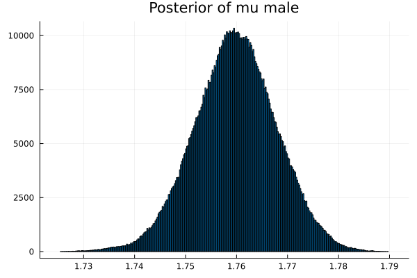
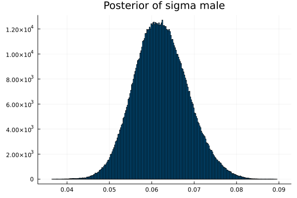
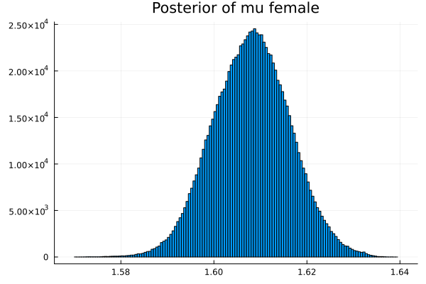
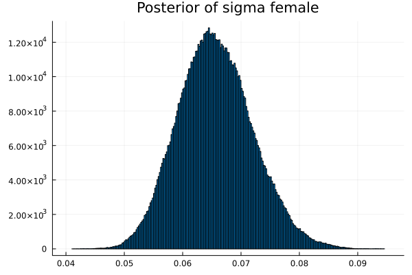
This is the limit on what we can know about the parameters without further specialized knowledge about the genders.

The best way to increase the accuracy of MCMC

The best way to increase the accuracy of MCMC is to get more datapoints.

For example: If we got 1000 datapoints instead of 100 datapoints, we can get much better results as seen below

$ julia --project=. bothgender02_turbo_d1000.jl
==================
turbonum is 0
┌───────────┬────────┬─────────┬────────┬────────┐
│ Parameter │ Mean   │ Stddev  │ 5.5%   │ 94.5%  │
├───────────┼────────┼─────────┼────────┼────────┤
│ μm        │ 1.76   │ 0.0497  │ 1.75   │ 1.77   │
│ σm        │ 0.0643 │ 0.00578 │ 0.0598 │ 0.0689 │
│ μf        │ 1.62   │ 0.00548 │ 1.62   │ 1.63   │
│ σf        │ 0.0533 │ 0.00327 │ 0.0492 │ 0.0573 │
└───────────┴────────┴─────────┴────────┴────────┘
error score is 0.0185
==================
turbonum is 1
┌───────────┬────────┬─────────┬────────┬────────┐
│ Parameter │ Mean   │ Stddev  │ 5.5%   │ 94.5%  │
├───────────┼────────┼─────────┼────────┼────────┤
│ μm        │ 1.76   │ 0.00372 │ 1.75   │ 1.77   │
│ σm        │ 0.0641 │ 0.00252 │ 0.0602 │ 0.0682 │
│ μf        │ 1.62   │ 0.0028  │ 1.62   │ 1.63   │
│ σf        │ 0.0528 │ 0.00189 │ 0.0498 │ 0.0559 │
└───────────┴────────┴─────────┴────────┴────────┘
error score is 0.0249
==================
turbonum is 2
┌───────────┬────────┬─────────┬────────┬────────┐
│ Parameter │ Mean   │ Stddev  │ 5.5%   │ 94.5%  │
├───────────┼────────┼─────────┼────────┼────────┤
│ μm        │ 1.76   │ 0.00257 │ 1.76   │ 1.76   │
│ σm        │ 0.064  │ 0.00181 │ 0.0611 │ 0.0669 │
│ μf        │ 1.62   │ 0.00205 │ 1.62   │ 1.62   │
│ σf        │ 0.0526 │ 0.00148 │ 0.0502 │ 0.0549 │
└───────────┴────────┴─────────┴────────┴────────┘
error score is 0.0278

Further increasing in fitness using specialized knowledge about genders

In a nutshell, the more we know about the characteristic of the gender of the students, the more we can further increase th fitness of the estimated parameters.

Let us suppose that we know the following about the genders of the students BEFORE we start the experiment.

The sigma_of_male_student is greater than sigma_of_female_student. In other words, the variation of the height of the male students is greater than the variation of the height of the female students.
mu_of_male_student - mu_of_female_student = 0.14 In other words the average height of the male students is 14 cm higher than the average height of the female students

We can represent it in the loglikelihood function as

    function loglikelihood(data::Vector,μm,σm,μf,σf)
        numofdatapoints = length(data)
        result=0.0
        @inbounds for k = 1:numofdatapoints
            mmm = 0.55*pdf(Normal(μm,σm),data[k])
            fff = 0.45*pdf(Normal(μf,σf),data[k])
            result += (  log(   mmm + fff   )     +
                         (μm > μf ? 0.0 : -1.0)   +
                         (σm > σf ? 0.0 : -1.0)   +
                         (-1.0 * min( abs((μm - (μf+0.14))/0.05),1.0 )  )
                      )
        end
        return result
    end

So our sourcecode is

# Filename is "bothgender04_turbo.jl"
# Directory is "/Users/ssiew/juliascript/MCMC_dir"
include("/Users/ssiew/juliascript/MCMC_dir/SimpleMCMC.jl")

using Distributions, StatsPlots, Statistics
using .SimpleMCMC
using StableRNGs,Distributions

const μm_actual = 1.76
const σm_actual = 0.0635
const μf_actual = 1.62
const σf_actual = 0.0559

ActualParameters = [μm_actual,σm_actual,μf_actual,σf_actual]

function generatedata(;numofdatum = 100)
    rng = StableRNG(12345)
    data = zeros(numofdatum)
    # 55% male with 1.76 m and std dev of 0.0635
    for k = 1:Int64(55//100*numofdatum)
        data[k] = rand(rng,Normal(μm_actual,σm_actual))
    end
    # 45% female with 1.62 m and std dev of 0.0559
    for k = (1+Int64(55//100*numofdatum)):numofdatum
        data[k] = rand(rng,Normal(μf_actual,σf_actual))
    end
    return round.(data,digits=2)
end

# Generate a numeric score so that we can compare how MCMC is performing
function errorscore(actual_parameter, estimated_parameter, scalingfactor, weighting)
    local temp
    temp = actual_parameter .- estimated_parameter
    temp = temp ./ scalingfactor
    temp = temp .^ 2
    temp = temp .* weighting
    return round(sum(temp),sigdigits=3)
end

function MCMC_example()

    data = generatedata()

    μm = Normal(1.6, 0.5)
    σm = Uniform(0.0,1.0)
    μf = Normal(1.6, 0.5)
    σf = Uniform(0.0,1.0)

    # Put all our parameters into a list
    ListOfParams = Distribution[μm,σm,μf,σf]

    # The loglikelihood function which returns the log(probability),
    # given a fixed mu and a fixed sigma, of the sequence of datapoints
    function loglikelihood(data::Vector,μm,σm,μf,σf)
        numofdatapoints = length(data)
        result=0.0
        @inbounds for k = 1:numofdatapoints
            mmm = 0.55*pdf(Normal(μm,σm),data[k])
            fff = 0.45*pdf(Normal(μf,σf),data[k])
            result += (  log(   mmm + fff   )     +
                         (μm > μf ? 0.0 : -1.0)   +
                         (σm > σf ? 0.0 : -1.0)   +
                         (-1.0 * min( abs((μm - (μf+0.14))/0.01),1.0 )  )
                      )
        end
        return result
    end

    local vec_μm,vec_σm,vec_μf,vec_σf
    local MaxTurboCycle = 2
    for TurboCycle = 0:MaxTurboCycle
        println("==================")
        println("TurboCycle is ",TurboCycle)
        p = MetropolisHastings_MCMC(
                data,
                ListOfParams,
                loglikelihood,
                samples=1_000_000,
                burnedinsamples=1000
        )

        # Next we need to display the histogram of the column p[:,1]
        # this is the shape of the posterior produced by MCMC
        vec_μm=vec(p[:,1])  # Convert a Matrix column into a 1-D Vector
        vec_σm=vec(p[:,2])  # Convert a Matrix column into a 1-D Vector
        vec_μf=vec(p[:,3])  # Convert a Matrix column into a 1-D Vector
        vec_σf=vec(p[:,4])  # Convert a Matrix column into a 1-D Vector
        #describe_paramvec("μ","mu",vec_μ)
        #describe_paramvec("σ","sigma",vec_σ)
        t = describe_multiparamvec([("μm","mu male",vec_μm),
                                ("σm","sigma male",vec_σm),
                                ("μf","mu female",vec_μf),
                                ("σf","sigma female",vec_σf)
                                ],savegraph=true)

        estimated = round.(t[:,2],sigdigits=3)

        println("error score is ",
            errorscore(
            ActualParameters,
            estimated,
            [0.01,0.01,0.01,0.01],
            [1/4,1/4,1/4,1/4]
            )
        )

        ListOfParams = Distribution[ Normal(round(t[k,2],sigdigits=3),round(t[k,3],sigdigits=3))  for k=1:4 ]
    end

    histogram2d(vec_μm,vec_σm,nbins=100,xlabel="mu male",ylabel="sigma male") |> display
    savefig("histogram2D_mu_male_sigma_male.png")
    histogram2d(vec_μf,vec_σf,nbins=100,xlabel="mu female",ylabel="sigma female") |> display
    savefig("histogram2D_mu_female_sigma_female.png")
    histogram2d(vec_μm,vec_μf,nbins=100,xlabel="mu male",ylabel="mu female") |> display
    savefig("histogram2D_mu_male_mu_female.png")
    histogram2d(vec_σm,vec_σf,nbins=100,xlabel="sigma male",ylabel="sigma female") |> display
    savefig("histogram2D_sigma_male_sigma_female.png")

end

# We call the main function to kick off the example
MCMC_example()

So here are the results

$ echo "This is the prompt on Terminal on MacOS"
$ cd /Users/ssiew/juliascript/MCMC_dir
$ julia --project=. bothgender04_turbo.jl

Starting Julia...
               _
   _       _ _(_)_     |  Documentation: https://docs.julialang.org
  (_)     | (_) (_)    |
   _ _   _| |_  __ _   |  Type "?" for help, "]?" for Pkg help.
  | | | | | | |/ _  |  |
  | | |_| | | | (_| |  |  Version 1.8.5 (2023-01-08)
 _/ |\__'_|_|_|\__'_|  |  Official https://julialang.org/ release
|__/                   |
==================
TurboCycle is 0
┌───────────┬────────┬─────────┬────────┬────────┐
│ Parameter │ Mean   │ Stddev  │ 5.5%   │ 94.5%  │
├───────────┼────────┼─────────┼────────┼────────┤
│ μm        │ 1.75   │ 0.0094  │ 1.73   │ 1.76   │
│ σm        │ 0.0718 │ 0.00942 │ 0.0592 │ 0.0889 │
│ μf        │ 1.61   │ 0.0094  │ 1.59   │ 1.62   │
│ σf        │ 0.0624 │ 0.00804 │ 0.0514 │ 0.0771 │
└───────────┴────────┴─────────┴────────┴────────┘
error score is 0.778
==================
TurboCycle is 1
┌───────────┬────────┬─────────┬────────┬────────┐
│ Parameter │ Mean   │ Stddev  │ 5.5%   │ 94.5%  │
├───────────┼────────┼─────────┼────────┼────────┤
│ μm        │ 1.75   │ 0.00542 │ 1.74   │ 1.76   │
│ σm        │ 0.0703 │ 0.00581 │ 0.0615 │ 0.0801 │
│ μf        │ 1.61   │ 0.00542 │ 1.6    │ 1.62   │
│ σf        │ 0.0621 │ 0.00496 │ 0.0544 │ 0.0703 │
└───────────┴────────┴─────────┴────────┴────────┘
error score is 0.712
==================
TurboCycle is 2
┌───────────┬────────┬─────────┬────────┬────────┐
│ Parameter │ Mean   │ Stddev  │ 5.5%   │ 94.5%  │
├───────────┼────────┼─────────┼────────┼────────┤
│ μm        │ 1.75   │ 0.00334 │ 1.74   │ 1.76   │
│ σm        │ 0.0698 │ 0.00432 │ 0.0631 │ 0.0769 │
│ μf        │ 1.61   │ 0.00334 │ 1.6    │ 1.62   │
│ σf        │ 0.0623 │ 0.00388 │ 0.0561 │ 0.0686 │
└───────────┴────────┴─────────┴────────┴────────┘
error score is 0.702