This is the first of a series of posts that I'm planning to upload during the upcoming weeks. The covered material is based on the notes that I've gathered during the time I've been using Julia for scientific computing.
The general idea behind the Laplace approximation is to approximate a well-behaved uni-modal function with an unnormalized Gaussian distribution. "Well-behaved" means that this function should be twice-differentiable and that most of its area under the curve should be concentrated around the mode.
To approximate , we first make a second-order Taylor expansion around its mode .
Let and consider the second-order Taylor expansion of around :
Note that , since , so we have:
Applying the exponential function on both sides yields:
As a result, to approximate we need two things:
- The mode of either or (which is the same).
- The second derivative of at .
Let's look at an example implemented in Julia.
The task is to find the Laplace approximation of the function:
We start by importing the packages that we will be needing:
using Plots, LaTeXStrings         # used to visualize the result
using Optim: maximize, maximizer  # used to find x₀
using ForwardDiff: derivative     # used to find h''(x₀)
We continue by defining the function
:
f(x) = (4-x^2)*exp(-x^2)
The next step is to find the mode
of
, i.e., the argument that maximizes the function
. For this, we will use the maximize function from Optim.jl, a Julia optimization package. The arguments expected by maximize are the function to be maximized and the endpoints of the interval along which the optimization will be performed. The returned object is a structure with several information from which we can extract the mode using the maximizer function.
x = range(-2, 2, length=100)
x₀ = maximize(x -> f(x), first(x), last(x)) |> maximizer
The final step is to find
, i.e., the second derivative of
at its mode
. ForwardDiff.jl is performant Julia package that implements the derivative method to perform automatic differentiation:
h(x) = log(f(x))
hꜛꜛ(x) = derivative(x -> derivative(h, x), x) # second derivative
Now we can bring everything together to define the Laplace approximation
of our original function
:
q(x) = f(x₀) * exp((1/2) * hꜛꜛ(x₀) * (x-x₀)^2)
Note the resemblance of this function with the one we derived above. Julia is pretty neat, huh?
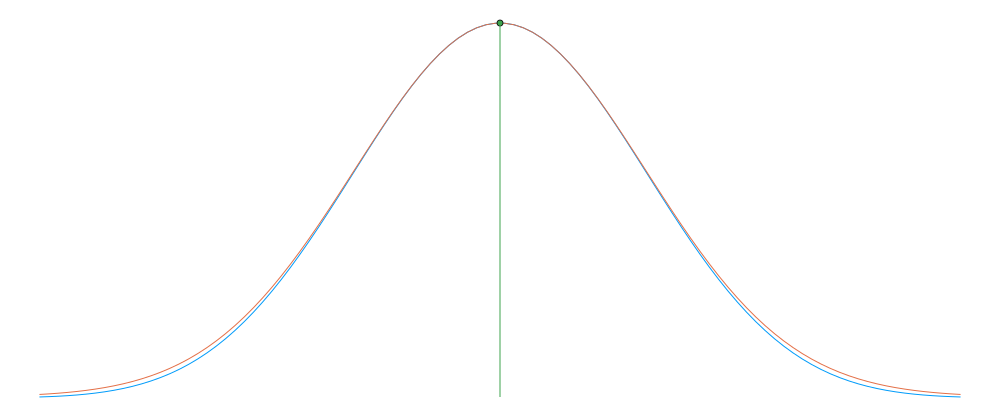
Finally, let's visualize the result:
plot( x, f, lab=L"f(x)= (4-x^2) \cdot e^{-x^2}", xlab=L"x", title=L"\textrm{Laplace~approximation}")
plot!(x, q, lab=L"q(x) = %$(f(x₀)) \cdot e^{\frac{%$(hꜛꜛ(x₀))}{2} x^2}")
sticks!([x₀], [f(x₀)], m=:circle, lab="")
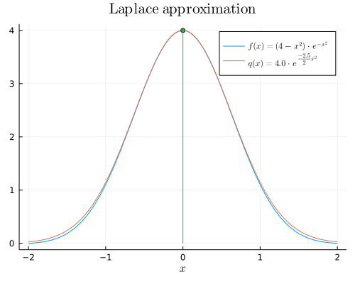
Pretty good approximation for this particular function!
To conclude, we showed how the Laplace approximation is a useful technique to approximate a well-behaved uni-modal function with an unnormalized Gaussian distribution, which is a well-understood and thoroughly studied quantity. Note, however, that if the function being approximated is not unimodal, or does not have it's mass concentrated around the mode, or is not twice-differentiable, then the Laplace approximation is not an adequate option. In part 2, I will go over the role that the Laplace approximation plays in the context of Bayesian inference.

Oldest comments (0)