GSoC 2022 -- Sparse Polynomial Zonotopes in JuliaReach

Hi there,

My Google Summer of Code (GSoC) journey has (again) come to an end, so here are some highlights.

whoami

I participated in GSoC already last year, working on IntervalLinearAlgebra.jl with David Sanders and Marcelo Forets as my mentors.

Given the experience was very positive, I decided this year to participate again. Given my interest in scientific computing and particularly rigorous computations, I ended up working in the JuliaReach organization with mentors Marcelo Forets and Christian Schilling.

The goals

Before getting into the nerdy parts, let's put some numbers on the table. My main goals for GSoC were mainly two-folded

• implement sparse polynomial zonotopes in LazySets.jl and reachability algorithms using those.
• Revamp RangeEnclosures.jl, to make it a working and useful package.

At the time of writing, I had 41 merged PRs related to GSoC. More details for each subgoal. I also had a JuliaCon talk and with Marcelo and Christian we are going to submit an extended abstract to the JuliaCon proceedings. Now let's dive into more details.

RangeEnclosures.jl

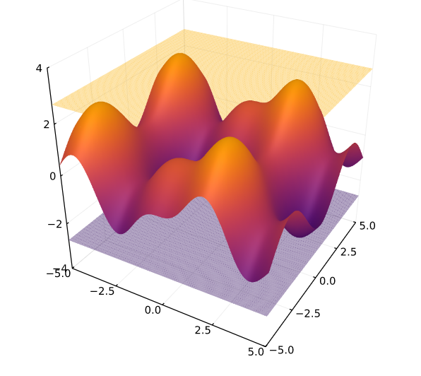
RangeEnclosures.jl is a package to rigorously bound function ranges. That is if you have a function $f : \mathbf{R}^n\rightarrow\mathbf{R}$ and you want to evaluate the function over a rectangle domain $X \subseteq \mathbf{R}^n$ you want to compute an interval $Y\supseteq f(X)$ . The following pictures give a visualization of the range bounding concept.

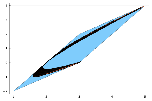
Now you may be wondering, isn't this what interval arithmetic does? Do you need a whole package for it? The answer is yes and no. It is true that interval arithmetic (assuming it's properly implemented) will give you a rigorous enclosure. That is, opening a Julia REPL and evaluating the function with IntervalArithmetic.jl will give you an interval which is probably bigger than the true range. Observe the following picture, where the function $f(x) = x^2 - 2x + 1$ is evaluated with interval arithmetic.

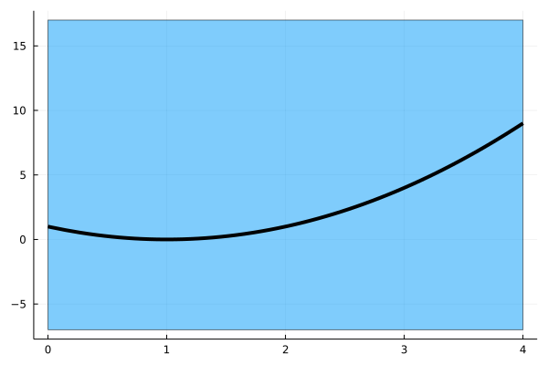
Why? Because interval arithmetic suffers from the so called dependency problem, which means that if your expression has the same variable repeated multiple times, then evaluating it with interval arithmetic will most likely introduce some overestimation.

So now the question is: how do you compute the range? The answer is: there is not one solution. There are several approaches, each one with its pros and cons

• Evaluate with interval arithmetic: this is good for simple functions and fast. But it is not recommended if you need tight enclosures.
• Use affine arithmetic: this makes the dependency problem milder, but can be worse for wider intervals
• Solve two global optimization problems: find the global maximum and global minimum, that gives you the range.
• Branch and bound: recursively split the domain into subdomains and evaluate on each subdomain until some ending condition is met, then take the union of all intervals
• use TaylorModels.jl
• etc.
• etc.

this is why we created RangeEnclosures.jl, it does not give you one method, but it is a flexible API that allows you to easily choose what approach you want to use in your application. It has some built-in algorithms, so it is battery included, but it also integrates algorithms implemented in different packages.

If you want to know more, check out the package documentation and/or my talk at JuliaCon.

(shameless advertisement: although not related to GSoC, I also gave another talk at JuliaCon about automated theorem proving in Euclidean geometry, check it out here)

Overall, I am pretty satisfied with how the package developed, sure there are still improvements that can be done, but the package should already be usable. If you ever need to bound the range of a function, you know where to go 😃

LazySets and Reachability Analysis

Before we go into the second goal, let's have a crash course in reachability analysis.

In one sentence: If you don't exactly know where you are at the beginning, reachability analysis tells you where you can possibly be at the end.

Now more formally, reachability analysis propagates rigorously uncertainty through dynamical systems. That is, if you know your initial state is in some set $X_0$ and you have a dynamical system $f(x, t)$ , generally represented by an ordinary differential equation, reachability analysis will give you a set $X_t$ guaranteed to contain the state of the system at time t. Again let's have a picture

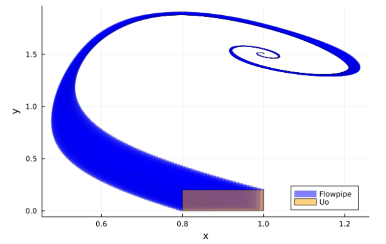
The yellow rectangle represent the initial set. You know your initial state is somewhere in that box, but you don't know exactly where. The picture shows the flowpipe modeling the evolution of the system. If you observe the picture carefully enough, you will notice it is composed by small blue sets, each one giving a set guaranteed to contain the system state at a given time instant.

Reachability analysis is a fairly new research area with an active research community. It also has a wide range of applications where safety is critical. For example, robotics and autonomous vehicles. You may not know exactly where your drone is at the beginning, but you still need to make sure it does not hit a tree at any point.

In Julia, there is ReachabilityAnalysis.jl, developed by Marcelo and Christian. This is a state-of-the-art library. If you want to learn more, make sure to checkout this workshop from last year JuliaCon.

Reachability and interval arithmetic.

Now you may be wondering, can I use interval arithmetic for this? The answer is (again) yes and no. Sure you could only use interval boxes, but this will (again) give huge overestimate. This is mainly for two reasons, the dependency problem we discussed before and the so called wrapping effect.

The idea of the wrapping effect is fairly simple, if you can only use interval boxes (i.e. rectangles) and your set is not a rectangle, then you need to overapproximate that, as the following picture demonstrates.

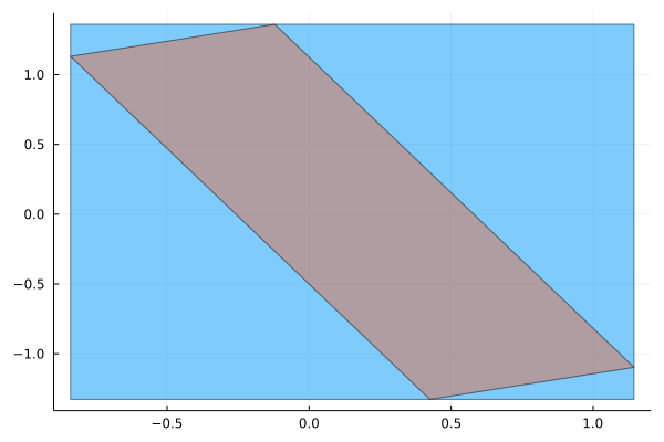
And now you may be asking, if I use the tightest interval box (called interval hull), wouldn't that be enough? Maybe, in some applications the interval hull would be enough. The problem is in general you do not get the interval hull. To understand this, look at the picture above again. You may notice you don't go straight from the initial state to the final one, but you take small steps in the middle. If you overapproximated by an interval box at every step, all these overapproximations would sum up and the final result will be much wider.

Beyond intervals: LazySets.jl

So we have seen interval and interval boxes are not accurate enough for reachability analysis. That's where LazySets.jl kicks in! We will not discuss here the lazy part, if you are interested have a look at this great paper from last year JuliaCon proceedings.

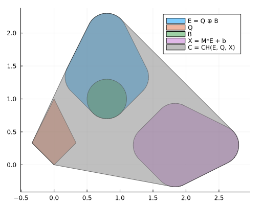
The idea of LazySets.jl is to represent other sets than intervals and compute efficiently operations with them. The following picture gives a quick overview of sets you can represent and manipulate in LazySets.jl

Using LazySets.jl we are able to get more accurate estimates in ReachabilityAnalysis.jl, for example the picture in the previous paragraph obtained using LazySets.jl and ReachabilityAnalysis.jl

Sparse Polynomial Zonotopes

Until recently, LazySets.jl could only represent convex sets. This is a limitation because, similarly to the wrapping effect for intervals, if your set is not convex, you need to overapproximate by a convex set and if you do this at each step of the reachability algorithm the final result might be pretty poor. The following picture visualizes the phenomenon.

To overcome this limitation, recently Sparse Polynomial Zonotopes were introduced. They are a novel set representation introduced in [1] that allows to manipulate also non-convex sets.

Most of my GSoC has been implementing sparse polynomial zonotopes in LazySets.jl. This was a very interesting challenge, because this new set representation and its application to reachability is still an active research area, with several open challenges.

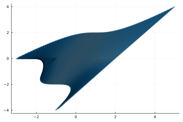
Roughly speaking, a sparse polynomial zonotope is a set whose coordinates can be parametrized by a multivariate polynomial. The following equation gives an example and the next plot visualizes the set.

During GSoC, I implemented sparse polynomial zonotopes in two flavours:

• SimpleSparsePolynomialZonotopes: a simplified version which can be more efficient but lead to wider sets
• SparsePolynomialZonotope: the "proper" polynomial zonotopes as described in [1].

I also implemented a plotting recipe (which allowed the pictures above) and several set operations. A summary of what has been implemented so far can be found at this epic issue.

References

• [1] Kochdumper, Niklas & Althoff, Matthias. (2019). Sparse Polynomial Zonotopes: A Novel Set Representation for Reachability Analysis.