GPU programming in DFTK.jl - GSoC 2022

Introduction

In 2022, I participated in the GSoC program. I worked on the DFTK libary, a molecular simulation package written in pure Julia. The aim of my project was to reduce runtime by offloading some computations to a local GPU.

Objectives

The goal of this GSoC is to build on the possibilities of GPU using Julia to allow specific computations in DFTK to be done faster. I am not running the entire code on GPU: instead, I focus on a few performance-critical operations whose structure can easily be adapted on GPU, as they mostly rely on matrix-vector operations. These matrix-vector operations aren't always blas-like matrix vector products, and can sometimes require to exploit sparsity (for example when computing FFTs): fortunately, these kind of operations usually are already available in vendor libraries. Since data transfer between CPU and GPU is very slow, I must isolate these key points in the code and make sure they form a series of instructions which can all be ran on the GPU, without any back-and-forth with the CPU. Non-essential operations can still be done on CPU.

The major guideline for this project is to try to build upon existing code and not make another implementation of DFTK: for code maintainability purpose, it is easier to have as much code in common as possible. By building on Julia's multiple dispatch, I should try to write code which is as generic as possible : the best version of the code would be one where the array type (CPU array or GPU array) is never specified, as the same code behaves similarly in both cases.

The last goal is to make an implementation that is not hardware-specific. Although I am running the code using CUDA because I have an NVIDIA GPU, it should also work using a AMD GPU for example. This can be done using some functionalities implemented in Julia's GPUArrays package, a low-level package giving the fundamental operations a GPU can execute.

Getting into the project

Getting into the project was a challenge in itself. I had already played around with Julia, but I needed to go much deeper in the possibilities of the language, especially concerning runtimes. It was the first time I take part in a project where runtime is one of the major aspect, and where the code base has to be structured around performance. Furthermore, it's the the first time I do a project involving massively parralelized computations: although I was aware of the possibilities GPUs offer in high performance computing and had some ideas about the GPU architecture, I had never really designed or adapted a code for GPU.

Finally, the last challenge was understanding the package in itself: DFTK is a molecular simulation library dedicated to plane-wave density-functional theory (DFT) algorithms. The most basic computation that can be done in DFT is solving the periodic Kohn-Sham equation. Getting to understand the chemical and physical models and the numerical algorithms used took some time: thankfully, the DFTK home page lists many references to get into this scientific background.

My experience with GPU programming

Getting into GPU programming is quite difficult, as I feel there are two levels of understanding and usage in Julia.

High level operations on vectors are easily adapted, thanks to Julia's polymorphism: most of these functions have already been adapted, so that mapping a function over a matrix, matrix-vector operations, eigen decompositions or cholesky factorization all have their GPU (in my case, CUDA) counterpart, making the code very direct and handy. Not everything can be adapted though, as scalar indexing is not allowed on GPU, since it performs very slowly. Therefore, most for loops have to be readapted or rewritten, which can be a real headache sometimes.

At a lower level and for more specific tasks, GPU programming requires to write kernels, which are functions which will be executed on the GPU. To write a proper kernel, one must be wary of the number and the way threads are used, but also of the separation between blocks. I experienced making some kernels to see what happens under the hood, and saw how difficult it can be to write parallel code for GPUs. I didn't code any for the DFTK project though, as they often require hardware-specific methods, and are a necessary divergence from the CPU code base.

One of the hardest thing I found with my high-level use of GPU programming is the understanding of error codes, as well as how to solve them. Scalar indexing errors were the most difficult to solve, as they are hard to track down and can be caused by almost anything. For example, some structure do not have specialized print method, so printing them requires to iterate through them, causing a scalar indexing error.

Another thing which took me way too long to fully understand is that all arguments in a GPU kernel must be isbits: generally, this means that every argument must have a fixed size and must not be a pointer to some other structure. This also applies to larger structure. A large structure in DFTK is the Model, which holds many physical specifications, such as a name, the atoms considered, their location in a lattice... Some of the fields in the models are isbits, for example the transition matrices used to change the coordinates in a which a vector is represented. Theses matrices are static matrices, and can be directly used in a kernel. However, some other fields are not isbits - the name is a string for example - and do not have to be on the GPU as they are not used in performance-heavy computations. Therefore, an instance of the model cannot be used or passed as an argument in a kernel.

This was actually more of a problem than I thought it would be, as it sometimes required to change the signature of a function for it to also work on GPU.

GPU programming in DFTK

The DFTK package implements various plane-wave density-functional theory (DFT) algorithms. Solving a problem using DFT comes to writing the Hamiltonian as a diagonal block matrix, and solving an eigenvalue problem for each block. One of the method used - and the only one I focused on - is LOBPCG, which is a matrix-free algorithm giving the largest eigenvalue of the eigenproblem λAx = Bx with A and B Hermitian, and B also definite-positive. The block version of this algorithm is used, which allows to compute several eigenpairs at a time, and reduces approximation errors.

The first step in the project was to make the implementation of LOBPCG GPU-compatible. The goal was to allow the input to be either a CPU array or a GPU array, and have the output be of the corresponding type. All major computations were already implemented in CUDA (eigen decomposition, cholesky decomposition, matrix inverse ...) so I didn't have to worry about very low-level functions. Instead, I focused on orchestrating the overall workflow of data to make sure critical operations were always done on the GPU and never transferred back on the CPU.

I quickly ran into some issues with an internal structure of data used to store arrays in blocks instead of concatenating them (which took up too much time in our case). These block structures were made using another Julia library which unfortunately isn't GPU compatible as it strongly uses the Julia's Array features (by Array, I refer to the Julia structure allowing computations to be done on CPU). I had to implement a custom BlockMatrix structure to be able to store both type of arrays - although to be honest, it didn't take much time as I simply retrieved the custom array structure used before that package was added in LOBPCG. After a few more tweaks, I finally had a first draft of LOBPCG, which could take either arrays or GPU arrays. Testing it for large structure quickly became difficult though: in a real DFT problem, it is not uncommon for the vectors considered to have thousands to hundreds of thousands of components. This makes explicitly defining the matrices A and B impossible, as it would take up too much memory space.

Since storing the matrices explicitly takes up an incredible amount of memory, DFTK stores the operators making up for the Hamiltonian blocks. Instead of giving LOBPCG a matrix A, we instead give an instance of a Hamiltonian block with a dedicated multiplication function. Applying the Hamiltonian mainly consists in applying the different operators describing the block. As such, each operator has an apply! function, yielding the result of the application of the operator to a given vector. My goal was therefore to adapt each operator so that the application could be GPU compatible.

At first, it started out slowly, with just a few operators describing very basic physical behaviors, such as a kinetic term (used to describe the free-electron Hamiltonian), or a local potential term. Getting these operators to work was not easy, as there are different object used at different levels. From a high-end user point of view, one only has to specify the different contributing terms in the problem (such as Kinetic(), AtomicLocal()...). For each of these terms, a Term object is build and stored in the the basis of plane waves: this Term object contains all the information about its impact on the system. Each of these Term can produce an operator, which is a function which can be applied to a vector. Both the Term and its associated operator had to be modified to be able to store and do computations with GPU arrays.

By the end of the GSoC, I managed to implement 4 terms out of 13 - and 3 more were already GPU-compatible, as they simply modified the Model and not the basis of plane waves. This allows to solve a linear DFT problem which is a first step: however, scaling up to the full problem requires solving non-linear equations, described for example by the exchange-correlation term. These additional terms will be much harder to write in a GPU-compatible way, either because they are very complex and were made using scalar indexing (meaning we probably would have to change the way they are created) or because they rely on external libraries.

The last big difficulty I faced was the way to distinguish between CPU arrays and GPU arrays. The generic way to offload an array A to the GPU is to call CuArray(A), and the way to get it back on the CPU is to call Array(A). However, in my case, the keyword for GPU offloading can change (CuArray, ROCArray...), and so I need a way to either store it or easily get it. I also need to create new arrays, by using these keywords.

At first, I thought I could use the similar function which builds an uninitialized array with a given element type and size, based upon the given source array. However, this doesn't cover all the cases, as some explicit conversions still need to take place. For example, using the QR decomposition doesn't yield two Array, but a object of type LinearAlgebra.QRCompactWYQ (for Q) and an Array (for R). I needed a way to replicate the conversion from QRCompactWYQ to Array but for GPU objects.

The solution to this was to make the plane wave basis parametric in the type of array used for computations: this allowed to easily retrieve it. It also makes high-end user input easier: to specify that computations should happen on GPU, one simply has to give the highest array type, such as CuArray, ROCArray... and not an initialized array. Therefore, the only difference in the code for end-user in when building the plane wave basis, with an optional argument.

A small benchmark

Although the GPU version of the code felt faster than the CPU one, I still needed to do some benchmarking to see what the real performance gain was.

In order to do a correct benchmark, I needed to have some sort of CPU parallelization, to see what were the performances in the best case scenarios. At first, I mostly played with three parameters:

• the number of CPU threads available for Julia. I could go up to 8, and got the best performances with the maximum number.
• the number of BLAS threads. From my testing, I got the best performances by setting a high number of threads, so I settle for the maximum (8).
• the number of FFT threads. I settle for the default number (1 thread).

The first tests were done using OpenBlas: however, following my mentors's advice, I switched to MKL which yielded much better results (some CPU computations went as much as 30% faster using MKL compared to OpenBlas).

For the following graph, I settled for a medium-sized example. I took a silicon supercell of parameters [4,4,2], and only considered three terms: the kinetic, local and nonlocal terms. I also disabled symmetries, as they are not implemented yet for GPUs. You can find the code here.

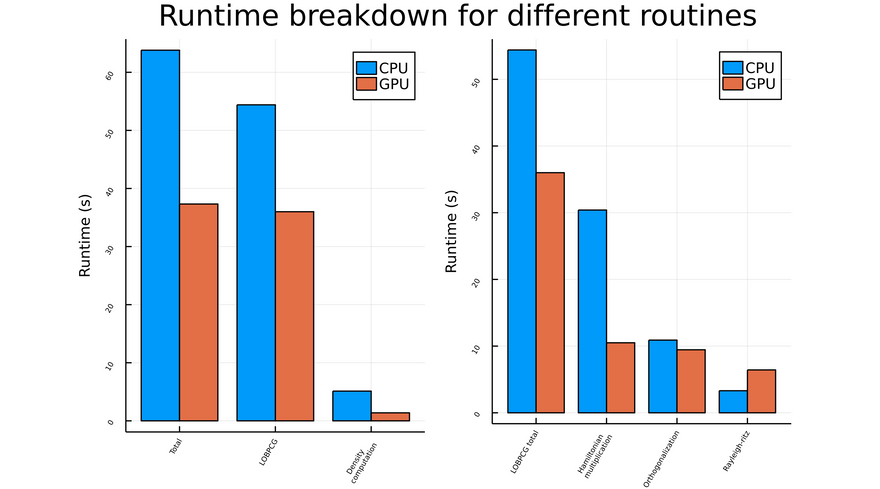
The overall runtime is reduced by approximately a factor of 1.7 for this example. Without suprises, LOBPCG takes up the most of computation time. It is worth noting that some computations made outside of LOBPCG, such as the density computation, can show significant improvement: however, these improvements do not contribute much, since it is LOBPCG which drives the overall runtime.

The LOBPCG runtime breakdown is shown on the graph to the right. A great speedup is achieved for the Hamiltonian multiplication, which makes sense as it consists in applying different operators to a vector (matrix-vector operations). There is still room for some improvement though, as some computations like the orthogonalization function barely show any sign of speedup; the fact that the rayleigh-ritz method takes longer on GPU than on CPU shows that I am not efficiently using the GPU's possibilities.

It is also worth noting that runtimes behave very differently from one example to another. For smaller systems, I noticed a speedup of up to 3, whereas for larger systems the speedup tends to fall down around 1.5: this is likely due to MKL's efficient parralelization for large systems. The GPU speedup we see is still interesting, especially considering that I have not written any tailored kernel specific for the algorithms, and have only build upon the existing functionalities in Julia.

Note: not all contributing terms were plotted in the graph, and there are many more functions making up for the full code. However, for the sake of simplicity, I have only represented major computations (computations taking more than a few seconds to execute) to show where speedups could happen.

Conclusion

This GSoC has been a great opportunity for me to learn more about GPU programming and the Julia language. Although a very challenging project, I took great pleasure in taking part of the development of the DFTK package. I especially enjoyed the conversations I had on Slack and Github with the community: thank you for your kindness and your patience. I would also like to thank my mentors for their steady help, support and guidance throughout the project period. Thanks for being available so often!