Creating Nice, Simple Geo-Plots From Scratch using Makie.jl

Introduction

It's quite a bit of work to make a plot that looks good. Phrases like "publication-quality" come up a lot in online discussions and one wonders what at what point a plot actually counts as publication-quality. Different journals, websites and people are all going to have different standards but, in my mind, if I have a plot that

1. has equations, labels and text that are all consistent with default LaTeX rendering, formats and fonts and ...
2. can be rendered using vector graphics if needed and ...
3. just in general isn't a complete eyesore ...

then I'm doing pretty well.

It's surprisingly hard to fulfill these requirements. Depending on the package, achieving items 1., 2. and 3. can be in essentially any order of difficulty. Makie.jl is a very promising plotting ecosystem, and in this short tutorial, I will demonstrate how the stock blocks can be used to make an equirectangular plot of Earth's landmasses at high resolution. More to the point, this plot will fulfill items 1., 2. and 3. with below-average inconvenience!

Packages

We will use CairoMakie as the Makie backend to give us vector graphics capabilities right away. Note that this post has been exported from a notebook, so the figures are PNGs, but it is easy to save a figure fig as, for example, a PDF via save("my_fig.pdf", fig). Item 2. already done!

We will also use GeoMakie and in particular GeoMakie.GeoJSON to make parsing the landmass data very easy.

using Makie, CairoMakie
using GeoMakie, GeoMakie.GeoJSON

Building The Axis

The general Makie workflow hierarchy is that plots (lines, heatmaps, contours ...) are stuck an Axis which is stuck on a Figure. We want a nice big figure with large text and plenty of padding on the sides to make room for labels, so let's start with that. In fact, we'll be making this figure several times, so let's put it in a function for easy regeneration.

function default_fig()
    Figure(
        resolution = (1920, 1080), 
        fontsize = 50,
        figure_padding = (100, 100, 100, 100)
    )
end

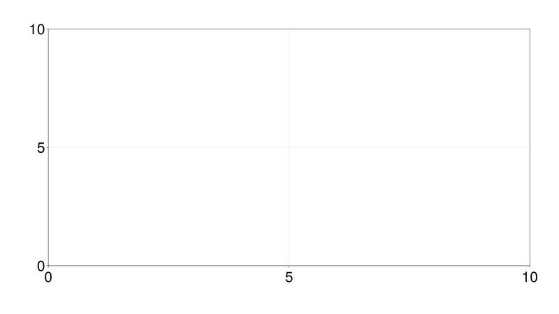
Arguably not very impressive yet, so let's add an Axis. All that is required of an Axis is that it is placed somewhere specific on a Figure. We want our axis in the first row and the first column of fig, so we simply pass fig[1, 1] to Axis.

fig = default_fig()
ax = Axis(fig[1, 1])
fig

At this point, we should ask a few things of our axis:

• It should have a title
• It should have the correct limits
• The tick marks should be placed where we want
• All numbers and text should have the correct formatting as per issue 1.

Fortunately, there is an easy way to demand LaTeX formatting, via L"my-latex-string". Therefore, to get a good-looking title, we can pass to axis something like title = L"\text{My Title}" with math and so on if needed.

What about limits? The world is truly our oyster here, but let's make a neat little box around the equator and Prime meridian. The region of interest will be from 20°W to 20°E by longitude and 20°S to 20°N by latitude. Hence, we can pass limits = (-20, 20, -20, 20).

And tick marks? Every 10° seems like a good separation. We'll use the default range constructor with xticks and yticks.

fig = default_fig()
ax = Axis(
    fig[1, 1],
    title = L"\text{The World, By Land}",
    limits = (-20, 20, -20, 20),
    xticks = -20:10:20,
    yticks = -20:10:20
)
fig

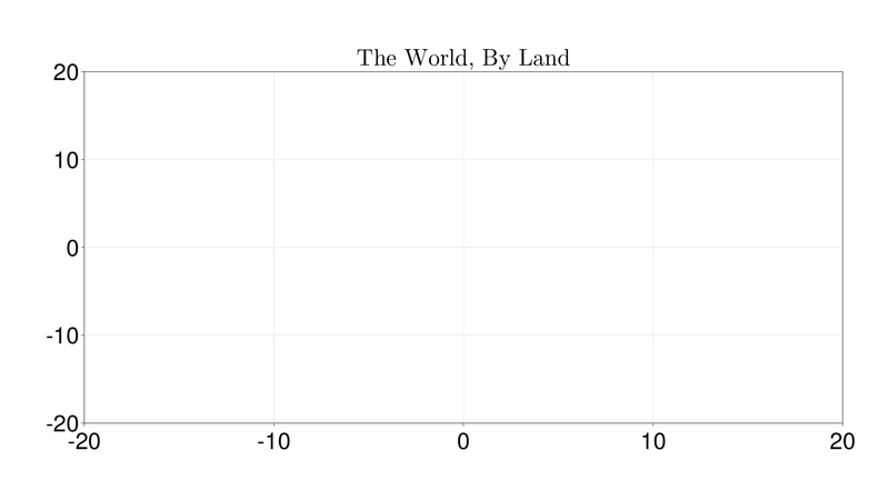
Now we're getting somewhere. The tick marks still don't have the correct font, and they also don't seem to be correctly referring to longitudes and latitudes. That is, -20 on the x axis should actually read 20°W and so on. The way to deal with this is with the handy xtickformat and ytickformat. This allows us to provide a map between the values of the ticks and the string that we actually want displayed.

A basic pattern for this is

xtickformat = values -> [f(value) for value in values]

where f(value) represents we want to actually do to a particular tick mark whose value is value. What do we want in this case? Well, if xtick < 0, we want it to be mapped to abs(xtick) °W with the L"" formatting and similarly for xtick > 0 and the yticks. This is accomplished with a basic if/elseif chain, with the one potential hiccup being that we need to use the % character to interpolate variables inside of L"".

These functions will map x and y ticks to the appropriate string.

function xtick_to_lon(value::Real)
    if value > 0 
        L"%$(abs(value)) \, \degree \mathrm{E}" 
    elseif value == 0 
        L"0\degree"
    elseif value < 0
        L"%$(abs(value)) \, \degree \mathrm{W}" 
    end
end

function ytick_to_lat(value::Real)
    if value > 0 
        L"%$(abs(value)) \, \degree \mathrm{N}" 
    elseif value == 0 
        L"0\degree"
    elseif value < 0
        L"%$(abs(value)) \, \degree \mathrm{S}" 
    end
end

Now we can get the right formatting.

fig = default_fig()

ax = Axis(
    fig[1, 1],
    title = L"\text{The World, By Land}",
    limits = (-20, 20, -20, 20),
    xticks = -20:10:20,
    yticks = -20:10:20,
    xtickformat = values -> [xtick_to_lon(value) for value in values],
    ytickformat = values -> [ytick_to_lat(value) for value in values]
)

fig

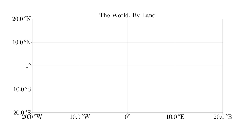
Hmm, the bottom left corner looks a bit cramped. It's always something, isn't it? Fortunately, we have the xticklabelpad and yticklabelpad to push the labels back a bit.

fig = default_fig()

ax = Axis(
    fig[1, 1],
    title = L"\text{The World, By Land}",
    limits = (-20, 20, -20, 20),
    xticks = -20:10:20,
    yticks = -20:10:20,
    xtickformat = values -> [xtick_to_lon(value) for value in values],
    ytickformat = values -> [ytick_to_lat(value) for value in values],
    xticklabelpad = 10.0,
    yticklabelpad = 10.0
)

fig

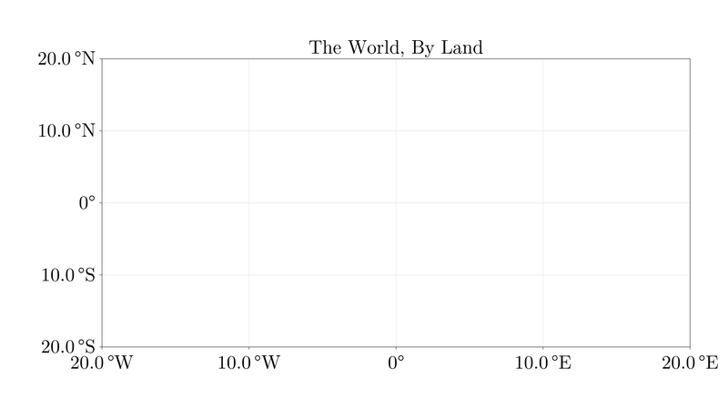
Add padding to taste, but it's looking pretty good!

Land spotted!

We will use Natural Earth Data since it is in the public domain and it has high resolution. The relevant repository is here. We're looking for the .geojson files; a 50 meter resolution should be enough. Simply download the raw data and pipe the result into GeoJSON.read to have a Makie-ready FeatureCollection.

url = "https://raw.githubusercontent.com/nvkelso/natural-earth-vector/master/geojson/"
landmass = download(url * "ne_50m_land.geojson") |> GeoJSON.read
# FeatureCollection with 1420 Features

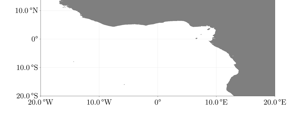
A FeatureCollection is easily plottable using the poly! command. We can choose the color using the many built-in named colorant options. Let's go for a classy gray.

poly!(ax, landmass, color = colorant"gray50")
fig

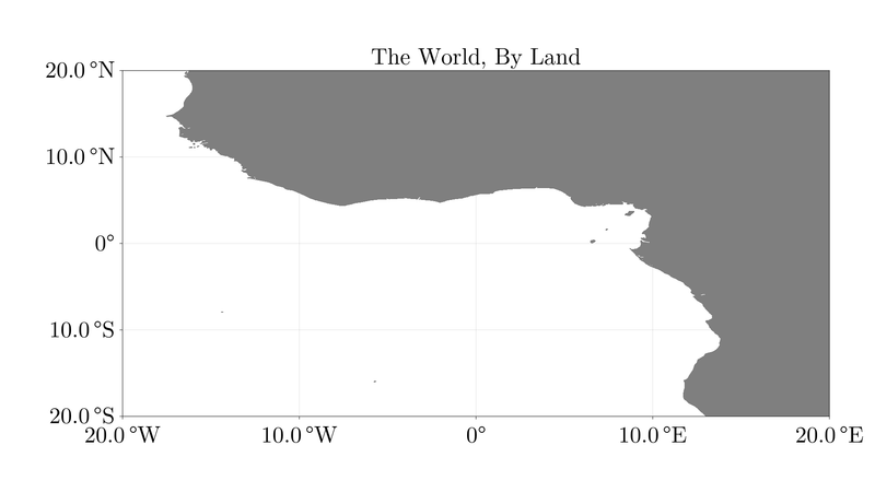
All of a sudden, Africa appears! Looks like the Gulf of Guinea to me, and we even have enough resolution to see the Cameroon Line.

The Axis we have cooked up forms a great baseline for more complicated plots. You can now easily add lines, polygons, and other plots on top of this for basic visualization.

Conclusion

We have created a basic template for equirectangular geo-plots with landmasses already filled in, and were only somewhat inconvenienced. Issues 1., 2. and 3. have been handled to my satisfaction. Job's done, good luck out there!