
This blog post first appeared in an ENCCS newsletter. ENCCS is the Swedish EuroCC center which aims to empower Swedish industry, academia and public sector to leverage HPC, AI, and HPDA efficiently and effectively, with a particular focus on EuroHPC resources.
This post gives an overview of Julia's features and capabilities for high performance computing (HPC) and presents a walkthrough on how to benchmark, optimize, parallelize and GPU-port a simple but realistic example problem. It builds on topics covered in the ENCCS workshop Julia for high-performance scientific computing.
To follow along with the code examples and do your own experiments you will need access to the Julia REPL. The official installation instructions provide a quick and painless way to install Julia on all major operating systems, but you can also run Julia in the cloud for a small cost via JuliaHub (who sponsorded the ENCCS workshop by giving participants free credits to run Julia on GPUs!). Code examples below can be copy-pasted into the Julia REPL. If you prefer an integrated development environment, there is an excellent Julia VSCode extension which is the prefered environment for many Julia developers.
To install the packages needed to run code found in this post, copy-paste the following dependency list into a file Project.toml in a new directory:
[deps]
BenchmarkTools = "6e4b80f9-dd63-53aa-95a3-0cdb28fa8baf"
CUDA = "052768ef-5323-5732-b1bb-66c8b64840ba"
Distributed = "8ba89e20-285c-5b6f-9357-94700520ee1b"
Plots = "91a5bcdd-55d7-5caf-9e0b-520d859cae80"
SharedArrays = "1a1011a3-84de-559e-8e89-a11a2f7dc383"
Then start Julia in the directory using the command julia --project which tells Julia to look for a Project.toml file in the current directory. Finally run the following commands inside the REPL to activate a new software environment and download the dependencies listed in Project.toml:
using Pkg
Pkg.activate(".")
Pkg.instantiate()
Introducing the toy problem
As an example numerical problem, we will consider the discretized Laplace operator which is used widely in applications including numerical analysis, many physical problems, image processing and even machine learning. Here we will consider a simple two-dimensional implementation with a finite-difference formula, which reads:
In Julia, this can be implemented as
function lap2d!(u, unew)
    M, N = size(u)
    for j in 2:N-1
        for i in 2:M-1
            unew[i,j] = 0.25 * (u[i+1,j] + u[i-1,j] + u[i,j+1] + u[i,j-1])
        end
    end
end
Note that we follow the Julia convention of appending an exclamation mark to functions that mutate their arguments.
We now start by initializing the two 64-bit floating point arrays u and unew, and arbitrarily set the boundaries to 10.0 to have something interesting to simulate:
M = 4096
N = 4096
u = zeros(M, N)
# set boundary conditions
u[1,:] = u[end,:] = u[:,1] = u[:,end] .= 10.0
unew = copy(u);
To simulate something that resembles e.g. the evolution of temperature in a 2D heat conductor (although we've completely ignored physical constants and time-stepping involved in solving the heat equation), we could run a loop of say 50,000 "time" steps and visualize the results with the heatmap method of the Plots package:
for i in 1:50_000
    lap2d!(u, unew)
    # copy new computed field to old array
    u = copy(unew)
end

using Plots
heatmap(u)
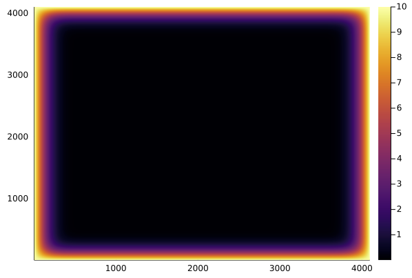
This might however take around an hour on a standard CPU, so it's time to start optimizing and later on parallelizing and GPU-porting our function! But first we need a way to benchmark our code.
Benchmarking
Base Julia already has the @time macro to print the time it takes to execute an expression. However, to get more accurate values it is better to rely on the BenchmarkTools.jl framework, which provides convenient macros for benchmarking:
-
@btime: quick timing, prints the time an expression takes and the memory allocated -
@benchmark: run a fuller benchmark on a given expression.
Let's try it:
using BenchmarkTools

@btime lap2d!(u, unew)
#  24.982 ms (0 allocations: 0 bytes)
Optimization
Before we start optimizing it is worth mentioning an important performance pitfall: multidimensional arrays in Julia are in column-major order like in Fortran, Matlab and R, but opposite to that of C/C++ and Python (numpy). If we were to mistakenly have the inner for-loop run over the second dimension (along rows) of the array (for i in 2:N-1; for j in 2:M-1; unew[i, j] = ...) this could increase the execution time by 2-3 orders of magnitude because of cache misses in every single inner loop iteration! The Julia manual contains a useful list of additional performance pitfalls and tips.
We first consider the @inbounds macro which eliminates array bounds checking within expressions. This can save considerable time, but should only be used if you are sure that no out-of-bounds indices are used. A good practice to ensure this is to use the eachindex method when iterating over collections. For example:
A = [1 2; 3 4];

for i in eachindex(A)
    println(i)
end
For the lap2d! function, we'll have to content ourselves with manually ensuring that no out-of-bounds errors can occur. The @inbounds macro can be inserted in front of an expression or a code block:
function lap2d!(u, unew)
    M, N = size(u)
    for j in 2:N-1
        for i in 2:M-1
            @inbounds unew[i, j] = 0.25 * (u[i+1,j] + u[i-1,j] + u[i,j+1] + u[i,j-1])
        end
    end
end
This should result in considerable speedup:
@btime lap2d!(u, unew)
#  15.205 ms (0 allocations: 0 bytes)
Another attempt at optimizing serial performance in Julia is to use the experimental @simd macro. This grants extra liberties to the LLVM compiler to allow loop re-ordering which in some cases can yield a speedup, although often the compiler is able to vectorize inner loops without the use of @simd and no speedup will be seen. Using @simd comes with a few requirements which you can see in the manual (type ?@simd in the REPL). For our Laplacian function, adding @simd to the inner-most loop does not improve performance on an AMD Epyc 7H12 CPU in the Vega EuroHPC supercomputer.
Parallelization
We now move on to parallelization. It's worth mentioning first that Julia has inbuilt automatic parallelism which automatically multithreads certain operations. Consider the multiplication of two large arrays:
A = rand(10000,10000)
B = rand(10000,10000)
A*B
If we run this in a Julia session and monitor the resource usage (e.g. via top on MacOS/Linux or the Task Manager in Windows) we can see that all cores on our computer are used!
The lap2d! function will not be automatically multithreaded, so we will first resort to the in-built Threads library. First let's see how many threads we have access to in our Julia session:
Threads.nthreads()
This will probably return 1, unless you have configured your Julia REPL, Jupyter Notebook kernel or VSCode Julia extension to use multiple threads. To start Julia with multiple threads, we need to add the -t/--threads flag when starting the REPL or set the Julia: Num Threads option in VSCode. The -t flag supports an auto keyword which automatically sets nthreads to the number of CPU threads on the machine.
After restarting a Julia session with e.g. 2 threads (julia -t 2), we can use the main multithreading approach of adding the Threads.@threads macro to the outermost for loop:
# Threads is in the standard library so append the module with a dot
using .Threads

function lap2d!(u, unew)
    M, N = size(u)
    @threads for j in 2:N-1
        for i in 2:M-1
            @inbounds unew[i,j] = 0.25 * (u[i+1,j] + u[i-1,j] + u[i,j+1] + u[i,j-1])
        end
    end
end
How efficiently does it parallelize?
@btime lap2d!(u, unew)
#  11.943 ms (11 allocations: 1.02 KiB)
A modest speedup, but not insignificant. Clearly the overhead of managing the threads balances the benefit of parallelization since the computation in the inner loop is very simple and fast. Adding more threads will also not help.
Another way to accomplish parallelization on a single computer (i.e. utilizing shared memory) is to use the SharedArrays package. A SharedArray is an array which is shared between threads in a shared-memory machine (in contrast to a DistributedArray which is distributed over multiple machines) but can be operated on with methods from the in-built Distributed module which handles message-passing parallelism between multiple concurrent Julia processes.
We can implement a new method for the lap2d! function which takes SharedArrays. To distribute the work in the double for-loop among parallel processes (workers), we add the @distributed macro to spawn independent workers and the @sync macro to synchronize the workers at the end:
using SharedArrays
using Distributed

function lap2d!(u::SharedArray, unew::SharedArray)
    M, N = size(u)
    @sync @distributed for j in 2:N-1
        for i in 2:M-1
            @inbounds unew[i, j] = 0.25 * (u[i+1,j] + u[i-1,j] + u[i,j+1] + u[i,j-1])
        end
    end
end
Even though we still intend to run our code on a single computer, the use of the Distributed module brings us into the territory of distributed computing which deserves a short discussion. Distributed enables us to create workers not only on single shared-memory machines but also on multiple interconnected workstations or across multiple nodes of a supercomputer. Each worker is an independent Julia process which receives work from the master process. One typical parallelization strategy with Distributed is to perform parallel reductions using constructs like @distributed (+) for i=1:N ; f(i) ; ... (summation with (+) can be replaced by any other reducer function). This divides work evenly between workers and is efficient for problems with fast inner loops. Another is to do parallel mapping with pmap in constructs like pmap(f, iterable), which is efficient to use with expensive function calls since it performs automatic load-balancing. More details about these methods can be found elsewhere.
Returning to our Laplacian function, we now need to create multiple workers. This can be done similarly to multithreading by adding the -p/--procs flag when we launch Julia, which also accepts an auto keyword. Alternatively, we can use methods from Distributed to manage worker processes within a Julia session:
using Distributed

println(nprocs())   # returns 1
addprocs(4)         # add 4 workers
println(nprocs())   # all processes, returns 5
println(nworkers()) # only worker processes, returns 4
rmprocs(workers())  # remove all worker processes
Let us add 4 worker processes, create new SharedArrays out of u and unew, and take advantage of multiple dispatch to measure the performance of the SharedArray-specialized method of the lap2d! function!
using Distributed
addprocs(4)

su = SharedArray(u);
sunew = SharedArray(unew);

@btime lap2d!(su, sunew)
#   14.106 ms (678 allocations: 31.56 KiB)
Not as efficient as using multithreading. The conclusion that can be drawn from these tests is that very simple calculations benefit little from parallelization due to the overhead in managing threads or processes.
GPU programming
Last but not least, we will turn our attention to porting our code to GPUs using the CUDA.jl package. For working on AMD or Intel GPUs there are corresponding packages AMDGPU.jl and oneAPI.jl, respectively. CUDA.jl offers both user-friendly high-level abstractions that require little programming effort and a lower level approach for writing kernels for fine-grained control. Unless you have an NVIDIA GPU on your own computer along with CUDA libraries, you will need to use JuliaHub or a GPU-powered supercomputer for the following code examples!
GPU programming with Julia can be as simple as using CuArray instead of regular Julia arrays. The CuArray type closely resembles Base.Array which enables us to write generic code which works on both types. The following code copies an array to the GPU, executes a simple operation on the GPU, and then copies the result back to the CPU:
using CUDA

A_d = CuArray([1,2,3,4])
A_d .+= 1

A = Array(A_d)
However, the overhead of copying data to the GPU makes such simple calculations very slow.
Let's see just how much performance one can get out of a GPU by performing a large matrix multiplication instead:
using BenchmarkTools

# array on CPU
A = rand(2^13, 2^13)
# array on GPU
A_d = CuArray(A)

@btime A * A
#   3.130 s (2 allocations: 512.00 MiB)
@btime A_d * A_d
#   15.190 μs (32 allocations: 640 bytes)
That's 200 times faster!
A powerful way to program GPUs with arrays is through Julia’s higher-order array abstractions. The simple element-wise addition we saw above, A_d .+= 1, is an example of this, but more general constructs can be created with broadcast, map, reduce, accumulate etc:
broadcast(A) do x
    x += 1
end

map(A) do x
    x + 1
end

reduce(+, A)

accumulate(+, A)
Moreover, the NVIDIA libraries contain precompiled kernels for common operations like matrix multiplication (cuBLAS), fast Fourier transforms (cuFFT), linear solvers (cuSOLVER), etc., and these kernels are wrapped in CUDA.jl and can be used directly with CuArrays:
# create a 100x100 Float32 random array and an uninitialized array
A = CUDA.rand(100, 100)
B = CuArray{Float32, 2}(undef, 100, 100)

# use cuBLAS for matrix multiplication
using LinearAlgebra
mul!(B, A, A)

# use cuSOLVER for QR factorization
qr(A)

# solve equation A*X == B
A \ B

# use cuFFT for FFT
using CUDA.CUFFT
fft(A)
Unfortunately, not all algorithms can be made to work with the higher-level array abstractions or preexisting kernels. In cases like our Laplacian operator it’s necessary to explicitly write our own GPU kernel.
In principle we could run our function as-is on a GPU by converting the input arrays to CuArrays and compile and run a GPU kernel using the @cuda macro (_d is often used for arrays living on the GPU device):
using CUDA

u_d = CuArray(u)
unew_d = CuArray(unew)

# WRONG!
@cuda lap2d!(u_d, unew_d)
However, the performance would be terrible because each thread on the GPU would be performing the same loop. What we have to do is to remove the loop over all elements and instead use the special threadIdx, blockIdx and blockDim functions to split array indices between computing elements on the GPU.
The following image shows how threads and thread blocks map to the hardware architecture of a GPU in the case of a 1D array:
(adapted from this CUDA tutorial, distributed under CC BY 4.0, Copyright (c) Artem Zhmurov and individual contributors)
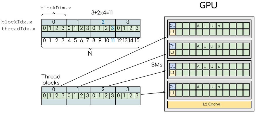
SM here stands for "streaming multiprocessor", the highest level of granularity in the GPU architecture. We see that for example index 11 in the array falls in block 2, has threadIdx=3 and that there are 4 threads per block. Thus, a for loop for i=1:N is usually replaced by i = threadIdx().x + (blockIdx().x - 1) * blockDim().x when writing a GPU kernel.
Let's see how our Laplacian function looks after porting it to the GPU:
@inbounds function lap2d_gpu!(u, unew)
    M, N = size(u)
    j = threadIdx().y + (blockIdx().y - 1) * blockDim().y
    i = threadIdx().x + (blockIdx().x - 1) * blockDim().x
    if i > 1 && i < N && j > 1 && j < M
        unew[i, j] = 0.25 * (u[i+1,j] + u[i-1,j] + u[i,j+1] + u[i,j-1])
    end
    return nothing
end
We use @inbounds for the same purpose as earlier, and we need the conditional to make sure we only use appropriate indices. Note also that GPU kernels always need to return nothing.
To launch this kernel we need to decide the number of threads and blocks in two dimensions (in each dimension, nthreads * nblocks should give the array size along that dimension). Setting the number of threads to 1 would be inefficient as only one GPU core per SM would be doing actual work. Setting the number of threads to the entire size of the array could be efficient, if only the GPU architecture supported it! Different families of GPUs come with different hardware limitations. We can call a function to see the maximum number of threads per block:
CUDA.attribute(device(), CUDA.DEVICE_ATTRIBUTE_MAX_THREADS_PER_BLOCK)
On an NVIDIA A100, a high-end GPU found on many current supercomputers (including Vega), the maximum number of threads is 1024. We can for example set the following numbers:
threads = (32, 32) # 32*32=1024
blocks = (N÷threads[1], M÷threads[2])
We launch the kernel with the @cuda macro and time it with @btime, but need to add CUDA.@sync to synchronize the GPU so that we don't measure only the kernel launch:
u_d = CuArray(u)
unew_d = CuArray(unew)

@btime CUDA.@sync @cuda blocks=blocks threads=threads lap2d_gpu2!($u_d, $unew_d)
#   248.392 μs (73 allocations: 4.25 KiB)
Around a factor of 45 faster than the multithreaded version!
But we might be able to do even better than this by using more threads in the x-dimension, since arrays in Julia are stored column-wise in memory:
threads = (256, 4)
blocks = (N÷threads[1], M÷threads[2])
@btime CUDA.@sync @cuda blocks=blocks threads=threads lap2d_gpu2!($u_d, $unew_d)
#   214.671 μs (26 allocations: 1.33 KiB)
Fortunately, the performance is not overly sensitive on this choice and thread configurations ranging from (128, 8) to (512, 2) all yield similar results.
GPUs typically perform significantly better in single precision, and some algorithms (e.g. molecular dynamics and neural networks) are sufficiently robust to handle reduced precision. Indeed, switching from double to single precision reduces the runtime by around 30-35\%:
unew_d = CuArray(Float32.(unew));
u_d = CuArray(Float32.(u));
@btime CUDA.@sync @cuda blocks=blocks threads=threads lap2d_gpu2!($u_d, $unew_d)
#   163.131 μs (26 allocations: 1.33 KiB)
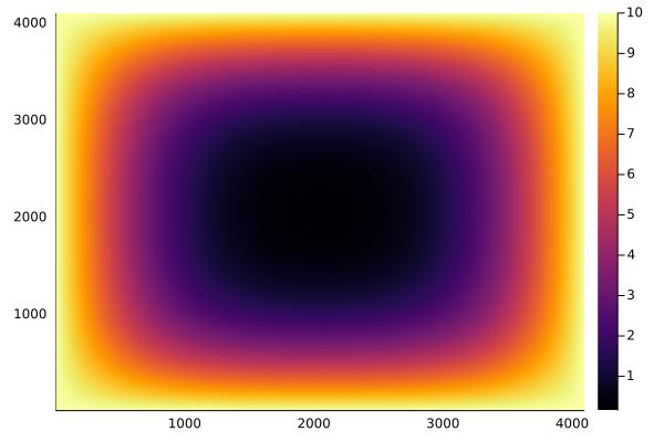
We can now easily afford to run a million iterations:
for i in 1:1_000_000
    @cuda blocks=blocks threads=threads lap2d_gpu!(u_d, unew_d)
    u_d = copy(unew_d)
end

heatmap(Array(u_d))
Further learning
More details on using Julia for HPC can be found in the ENCCS Julia lesson on which this post is based. There is also a large and rapidly growing number of online learning resources for Julia, some of which are listed on https://julialang.org/learning/. Finally, anyone interested in hearing about what's happening in the world of Julia should consider attending the free online JuliaCon 2022 conference!

Oldest comments (1)
Thanks! This is such a nicely explained article. It is very helpful for beginners like me to understand how Julia can be made to work optimally for GPUs and HPCs (even though I don't think I will ever get access to any HPC😅)
Please continue to post such articles where an equation is formulated into code that is optimized for Julia programming environments.