Steven Siew

Posted on Mar 12 • Updated on Mar 16

How to use Matrices to perform Simple Least Square fitting of experimental data

Assumptions
In this article I assume that You know

How to add a package to Julia
What the equation of a straight line is
What a quadratic equation is
What an XY graph is
What a Matrix is
The basic idea of what an inverse of a Matrix is
The basic idea of what a transpose of a Matrix is
Basic maths. Addition Subtration. Multiplication. Division. Power.

Let's make things simple. Let's just say that you are a Medical Researcher and you are performing an experiment. You want to measure a person's

Body Mass Index (BMI)
What percentage of the population in that BMI value has Type 2 Diabetes (You get this number from Medical Census)

You would have an XY graph where

X axis is the BMI
Y axis is the percentage of population in that BMI value that has Type 2 Diabetes

You want to get a linear equation of

Y = M * X + C where both M and C are numeric constants

and both variable X and Y are of various values

In this article, the actual values of X and Y does not matter. What I wanted to show is how to get the value of M and C using matrices in Julia.

First thing we need to do is to get some raw data. Rather then getting REAL DATA, we can just generate them using code from another article of mine earlier.

Let's write some code to generate experimental data X and Y

using Distributions,StableRNGs

#=
We want to generate Float64 data deterministically
=#

function generatedata(formula;input=[Float64(_) for _ in 0:(8-1)],seed=1234,digits=0,
    preamble="rawdata = ",noisedist=Normal(0.0,0.0),verbose=true)
    vprint(verbose,str) = print( verbose == true ? str : "")
    local myrng = StableRNG(seed)
    local array = formula.(input) + rand(myrng,noisedist,length(input))
    if digits > 0
        array = round.(array,digits=digits)
    end
        vprint(verbose,preamble)
    # Now print the begining array symbol '['
    vprint(verbose,"[")
    local counter = 0
    local firstitem = true
    for element in array
        if firstitem == true
            firstitem = false
        else
            vprint(verbose,",")
        end
        counter +=1
        if counter % 5 == 1
            vprint(verbose,"\n  ")
        end
        vprint(verbose,element)
    end
    vprint(verbose,"]\n")
    return array
end

M_actual = 0.4
C_actual = 0.3
f(x) = M_actual * x + C_actual 
numofsamples = 3
X = [ Float64(_) for _ in 0:(numofsamples-1)]
Y = generatedata(f,input=X,digits=2,noisedist=Normal(0.0,0.2),preamble="Y = ")
print("\n\nX = ",X,"\nY = ",Y,"\n\n")

and the output is

Y = [
  0.4,0.88,0.76]


X = [0.0, 1.0, 2.0]
Y = [0.4, 0.88, 0.76]

So we now have three equations (using Y = M * X + C )

0.40 = M * 0.0 + C
0.88 = M * 1.0 + C
0.76 = M * 2.0 + C

we can now rewrite the three equations as

0.40 = M * 0.0 + C * 1.0
0.88 = M * 1.0 + C * 1.0
0.76 = M * 2.0 + C * 1.0

Because multiplying anything by one changes nothing.

Next we change the order of the terms on the right hand side

0.40 = C * 1.0 + M * 0.0 
0.88 = C * 1.0 + M * 1.0 
0.76 = C * 1.0 + M * 2.0

Next we change the order of the multiplication

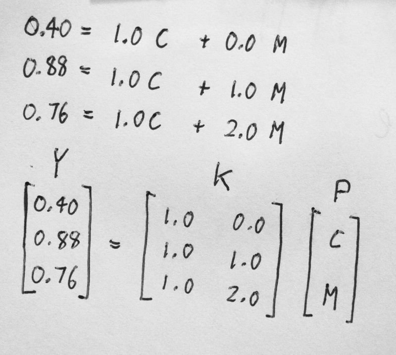
0.40 = 1.0 * C + 0.0 * M
0.88 = 1.0 * C + 1.0 * M
0.76 = 1.0 * C + 2.0 * M

Now we got it in a form that can be easily converted to Matrix format.

We shall use the following

Y to represent [ 0.4, 0.88, 0.76 ]
K to represent [ 1.0 0.0; 1.0 1.0; 1.0 2.0 ]
P to represent [ C , M ]

julia> K = [ 1.0 0.0; 1.0 1.0; 1.0 2.0 ]
3×2 Matrix{Float64}:
 1.0  0.0
 1.0  1.0
 1.0  2.0

So in Matrix form we have Y = K P
Where

K is the 3x2 matrix form of X
P is the 2x1 matrix form of the parameters C and M

Here is my rough sketch on paper

Now that we got it in Matrix format, all we need to do is to solve for P

This is the WRONG WAY to do it

Show wrong way to solve for P

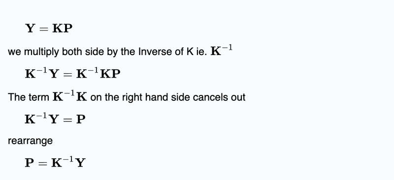
And here is why it is wrong!

julia> K = [ 1.0 0.0; 1.0 1.0; 1.0 2.0 ]
3×2 Matrix{Float64}:
 1.0  0.0
 1.0  1.0
 1.0  2.0

julia> inv(K)
ERROR: DimensionMismatch: matrix is not square: dimensions are (3, 2)
Stacktrace:
 [1] checksquare
   @ /Applications/Julia-1.10.app/Contents/Resources/julia/share/julia/stdlib/v1.10/LinearAlgebra/src/LinearAlgebra.jl:241 [inlined]
 [2] inv(A::Matrix{Float64})
   @ LinearAlgebra /Applications/Julia-1.10.app/Contents/Resources/julia/share/julia/stdlib/v1.10/LinearAlgebra/src/dense.jl:911
 [3] top-level scope
   @ REPL[3]:1

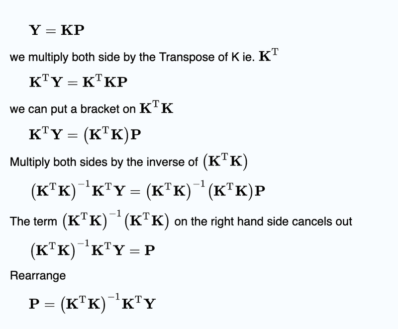
And this is the correct way to do it.

Let's write some code to implement our solution

"""
Provide the solution to the linear Least Square
"""
function linearLSQ(xarray,yarray)
    len_xarray = length(xarray)
    len_yarray = length(yarray)
    if len_xarray != len_yarray
        println("Error in function linearLSQ: length of xarray != length of yarray")
        return nothing
    end
    # Let's create the K Matrix
    K = zeros(len_yarray,2) # a len*2 matrix
    for i = 1:len_yarray
        K[i,1] = 1.0
        K[i,2] = xarray[i]
    end
    # Dont forget to reshape cases from a 1D vector yarray into a len*1 column matrix Y
    local Y = reshape(yarray,len_yarray,1)
    # In Julia K' is the Transpose of K
    P = inv(K'*K) * K' * Y
    return P
end

solution = linearLSQ(X,Y)
println("The estimate for C is ",solution[1])
println("The estimate for M is ",solution[2])

when we run it, we have the solution

The estimate for C is 0.5
The estimate for M is 0.17999999999999994

The reason we do not get the correct values is because we only have 3 experimental samples from our experimental data. We can get a better estimate if we do the experiment again with 100 samples.

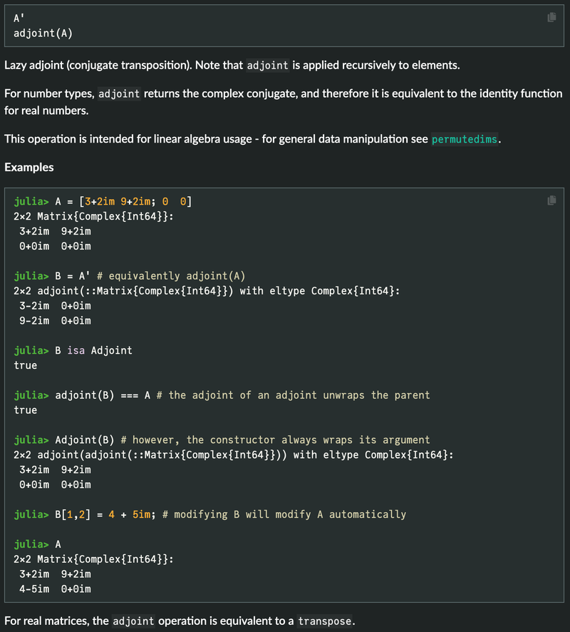
Also those of you who is observant will noticed that I use the Adjoint operator and not the transpose operator. This is because when used on REAL NUMBER matrices the adjoint operator is the same as a Transpose operator.

Let's do the experiment again with 100 samples this time

numofsamples = 100
X2 = [ Float64(_) for _ in 0:(numofsamples-1)]
Y2 = generatedata(f,input=X2,digits=2,noisedist=Normal(0.0,0.2),preamble="Y = ")

solution2 = linearLSQ(X2,Y2)
println("The estimate for C is ",solution2[1])
println("The estimate for M is ",solution2[2])

And the results are

Y = [
  0.4,0.88,0.76,1.24,1.76,
  2.16,2.72,3.08,3.21,3.52,
  4.12,5.03,5.07,5.42,6.01,
  6.14,6.78,7.23,7.49,7.91,
  8.21,8.68,8.91,9.48,9.99,
  10.37,10.9,10.85,11.43,11.89,
  12.28,12.48,13.14,13.71,13.92,
  14.42,14.64,15.09,15.52,15.75,
  16.4,16.59,16.86,17.38,18.02,
  18.11,18.57,19.2,19.66,19.71,
  20.06,20.79,21.18,21.2,21.5,
  22.48,22.67,22.89,23.25,24.0,
  24.1,24.9,25.33,25.52,26.22,
  26.31,27.13,27.52,27.18,27.97,
  28.28,28.86,28.99,29.43,29.69,
  30.45,30.59,31.16,31.56,31.85,
  32.15,32.71,33.1,33.08,34.23,
  34.39,34.96,35.27,35.39,35.72,
  36.07,36.68,36.96,37.74,37.71,
  38.09,38.82,39.11,39.53,40.37]
The estimate for C is 0.23681584158414637
The estimate for M is 0.4009188718871888

Now the estimated value for M is almost spot on but the estimated value for C is a bit off.

Using linear least square to predict/interpolate the next value in the sequence.

If the values are subject to only a little bit of noise, we can use linear least square to predict the next value in the sequence. For example:

numofsamples = 3
X3 = [ Float64(_) for _ in 0:(numofsamples-1)]
Y3 = generatedata(f,input=X3,digits=2,noisedist=Normal(0.0,0.02),preamble="Y = ",verbose=false)

println("\n\nX3 = ",X3,"\nY3 = ",Y3,"\n\n")

"""
Interpolate the next value in the sequence
using linear interpolation
"""
function LSQ_linear_nextseq(data; verbose=false)
    len = length(data)
    day = [ _ for _ in 0:(len-1)]

    #=
    using the Ordinary Least Squares Algorithm
    https://en.wikipedia.org/wiki/Linear_least_squares
    https://en.wikipedia.org/wiki/Ordinary_least_squares
    =#
    K = zeros(len,2) # a len*2 matrix
    for i = 1:len
        K[i,1] = 1.0
        K[i,2] = day[i]
    end
    # Dont forget to reshape cases from a 1D vector into a len*1 column matrix
    P = inv(K'*K) * K' * reshape(data,len,1)
    linear_func(t) = P[1] + P[2] * t
    next_value_in_sequence = linear_func(len)

    linear_param_rounded = round.(P,digits=4)
    if verbose
        println("linear model is $(linear_param_rounded[1]) + $(linear_param_rounded[2]) * t")
    end
    return next_value_in_sequence
end

println("The next value in the sequence is interpolated as ",
LSQ_linear_nextseq(Y3,verbose=true))

with the result

X3 = [0.0, 1.0, 2.0]
Y3 = [0.31, 0.72, 1.07]


linear model is 0.32 + 0.38 * t
The next value in the sequence is interpolated as 1.4600000000000002

So that is how to predict/interpolate the next value in the sequence but what about the previous value in the sequence? The easiest way is just to reverse the array and call the next value in the sequence again.

"""
Interpolate the previous value in the sequence
using linear interpolation
"""
function LSQ_linear_prevseq(data; verbose=false)
    newdata = reverse(data)
    value = LSQ_linear_nextseq(newdata)
    return value
end

Quadratic Least Squares

Linear Least Squares is basically modelling the data with a STRAIGHT LINE. But straight line is not the only way you can model experimental data. In high school we learn about quadratic equaion like this

Y = A * X^2 + B * X + C
or
Y = C + B * X + A * X^2

Using the data from https://en.wikipedia.org/wiki/Ordinary_least_squares (see picture below)

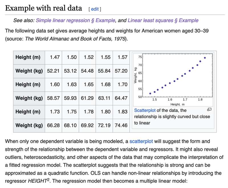
Here is the code

X4 = [ 1.47,1.50,1.52,1.55,1.57,1.60,1.63,1.65,
       1.68,1.70,1.73,1.75,1.78,1.80,1.83 ]

Y4 = [ 52.21,53.12,54.48,55.84,57.20,58.57,
       59.93,61.29,63.11,64.47,66.28,68.10,69.92,
       72.19,74.46 ]

"""
Provide the solution to the quadratic Least Square
"""
function quadLSQ(xarray,yarray)
    len_xarray = length(xarray)
    len_yarray = length(yarray)
    if len_xarray != len_yarray
        println("Error in function linearLSQ: length of xarray != length of yarray")
        return nothing
    end
    # Let's create the K Matrix
    K = zeros(len_yarray,3) # a len*3 matrix
    for i = 1:len_yarray
        K[i,1] = 1.0
        K[i,2] = xarray[i]
        K[i,3] = xarray[i]^2.0
    end
    # Dont forget to reshape cases from a 1D vector yarray into a len*1 column matrix Y
    local Y = reshape(yarray,len_yarray,1)
    P = inv(K'*K) * K' * Y
    return P
end

solution4 = quadLSQ(X4,Y4)
print("\n\n")
println("The estimate for C is ",solution4[1])
println("The estimate for B is ",solution4[2])
println("The estimate for A is ",solution4[3])

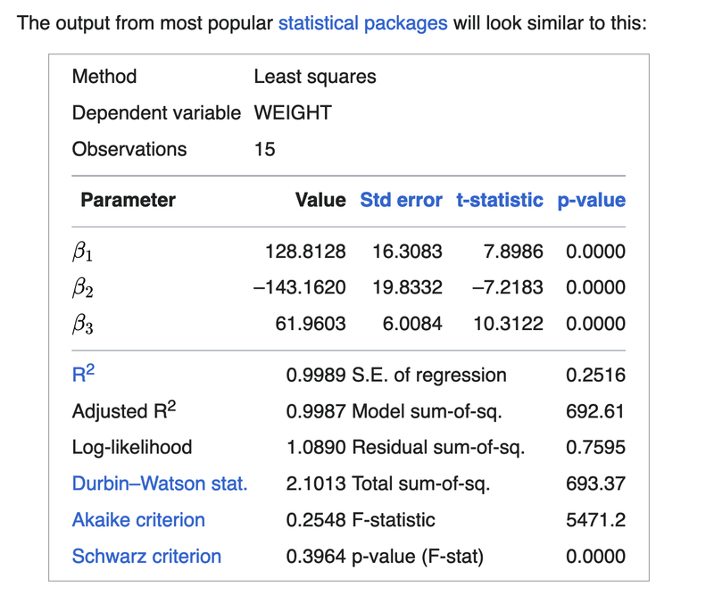
With the output

The estimate for C is 128.81280358089134
The estimate for B is -143.16202286910266
The estimate for A is 61.96032544388436

Compare our result with the result on the wikipedia page below

Julia Community 🟣

How to use Matrices to perform Simple Least Square fitting of experimental data