Floating-point accuracy visualization example: the ULP error for each math function coming with Julia

Introduction

How about visualizing the discrepancy between the exact value of a univariate real function, such as the sine, and the approximate value that is returned by a call such as sin(0.3). By putting an interval that subsets the domain of the function on the x-axis of a plot, and the value of this discrepancy, the error onto the y-axis of the same plot, it might be possible to tell on which part of the function's domain is the implementation less accurate than on other parts. That is, it might be possible to read the worst-case regions for the approximation off the plot.

I choose the error measured in units in the last place/units of least precision (ULPs) as the type of error to visualize here. Other types of error that are often used are absolute error, which is not usually appropriate for floating-point numbers, and relative error, which has these drawbacks to measuring the error in ULPs:

• it is usually less immediately useful and less intuitive

• plotting software tends to have trouble with the tiny values

One advantage of the error in ULPs is that it has some convenient and easy interpretations in the context of floating-point numbers. For example:

• If the error between the exact value and the approximate (floating-point) value is less than half, the approximate value is the number closest to the exact value among the numbers belonging to that floating-point representation. The technical term is correctly rounded.

• If the error is merely less than one, the approximate value is one of the two floating-point numbers closest to the exact value. The technical term is faithfully rounded (although faithful rounding is not technically a rounding).

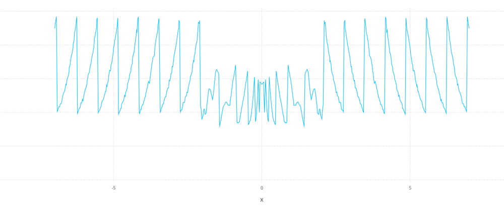
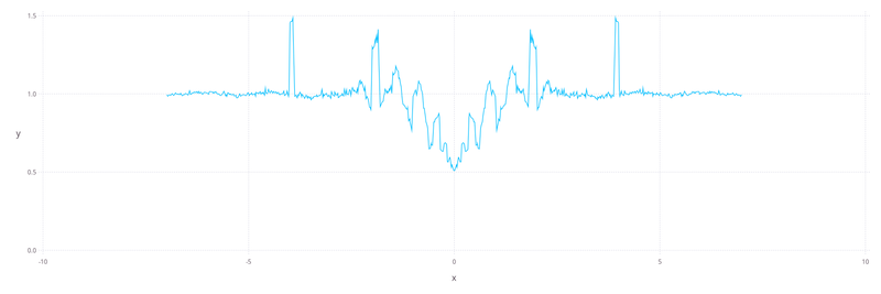
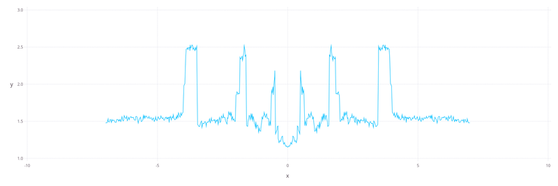
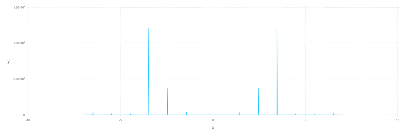
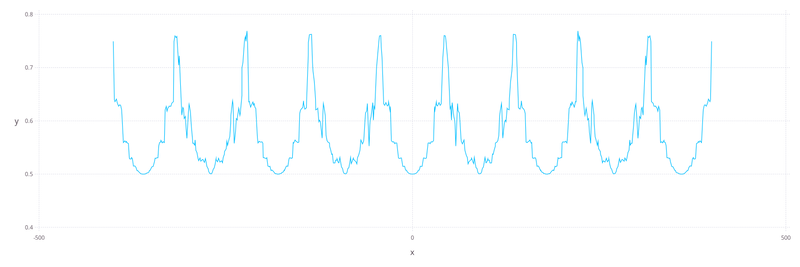
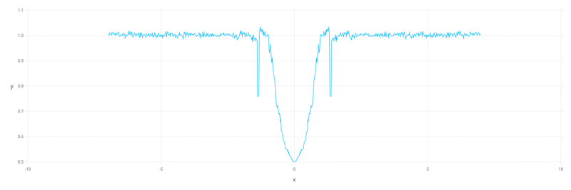
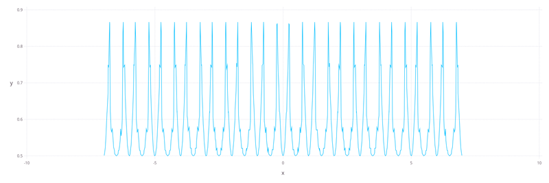
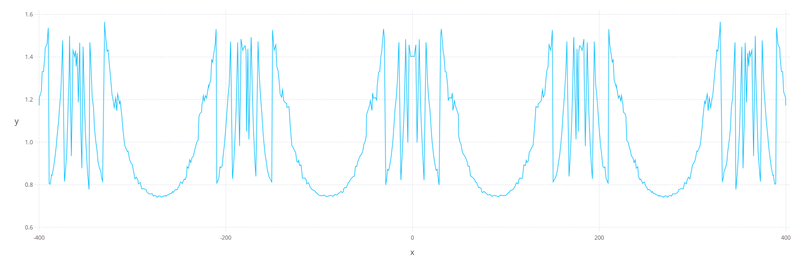
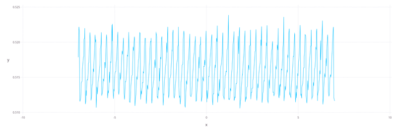
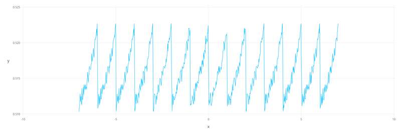
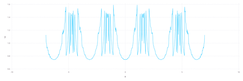
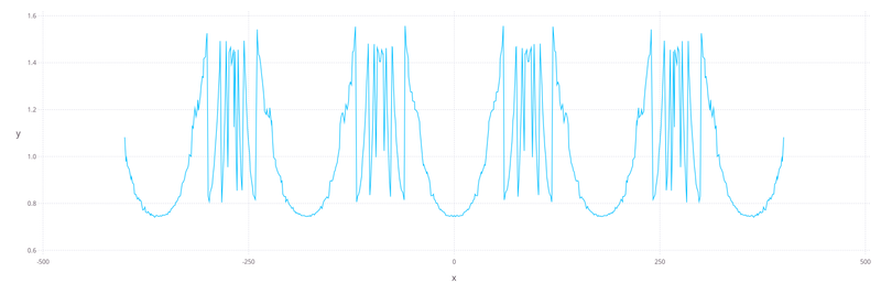
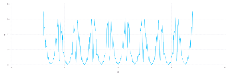
If we tried to, say, evaluate the error in ULPs on an evenly-spaced grid on the chosen interval, the plot would just like like noise if each evaluation was plotted as a data point. However, given that the worst cases are what is most interesting, it might be possible to achieve a comprehensible visualization by giving up on visualizing the best cases. In other words, we're interested in the upward spikes of the error, and by eliding the downward spikes it might be possible to make the plot a lot less noisy.

To accomplish this, the approach I choose here is vaguely similar to downsampling/decimation, from signal analysis: take n values, where n is some large positive integer, and represent them on the plot by an aggregate value: the maximum value among the n points (in this case). In a signal analysis context, it is also common to apply a lowpass filter to reduce noise/high-frequency components of the signal, before the decimation itself. This helps prevent artifacts in the resulting output. In this case, a sliding window maximum seems like an appropriate lowpass filter to smooth out the data before decimation, to prevent artifacts.

Julia app on Github

The app used for creating these visualizations is published on Github:

• https://github.com/nsajko/VisualizeULPError.jl

NB:

• Neither the package, nor the app it exposes, are registered as of writing this.

• Probably should move the Git repository from my personal namespace to the JuliaMath organization on Github.

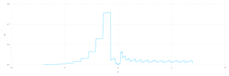
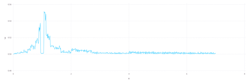
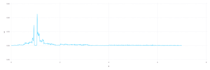
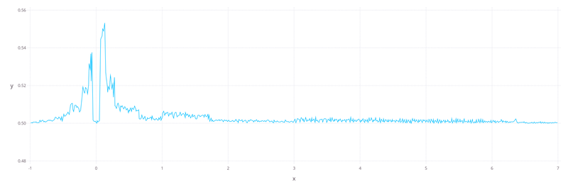
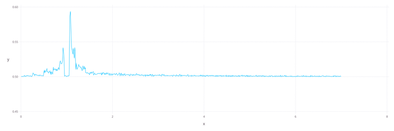
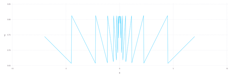
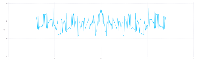
The plots

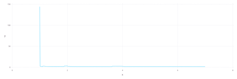
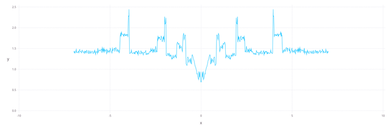
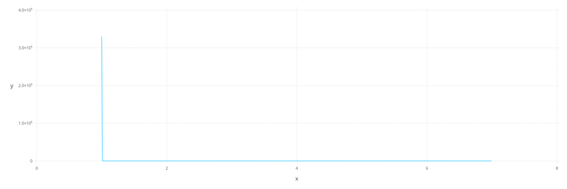
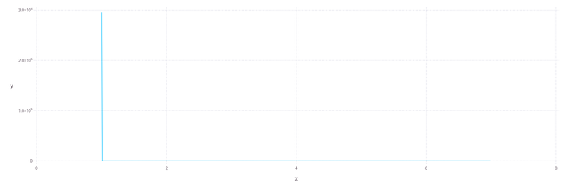
Might be useful to both contributors and users of Julia to better understand where there's room for improvement in the current implementations. In the cases of some functions, though, the worst case error spikes are difficult or impossible to fix efficiently, without reaching for some arbitrary-precision implementation like MPFR (BigFloat) or Arb.

acos

acosd

acosh

acot

acotd

acoth

acsc

acscd

acsch

asec

asecd

asech

asin

asind

asinh

atan

atand

atanh

cos

cosc

cosd

cosh

cospi

cot

cotd

coth

csc

cscd

csch

deg2rad

exp

exp10

exp2

expm1

log

log10

log1p

log2

rad2deg

sec

secd

sech

sin

sinc

sind

sinh

sinpi

tan

tand

tanh

tanpi

Miscellaneous

Connected discussions

Julia Discourse:

• https://discourse.julialang.org/t/new-on-forem-floating-point-accuracy-visualization-example-the-ulp-error-for-each-math-function-coming-with-julia/135392?u=nsajko

Connected PRs

• Julia itself

  • https://github.com/JuliaLang/julia/pull/59031
  • https://github.com/JuliaLang/julia/pull/59087
  • https://github.com/JuliaLang/julia/pull/59097

• Julia package LogExpFunctions.jl

  • https://github.com/JuliaStats/LogExpFunctions.jl/pull/99
  • https://github.com/JuliaStats/LogExpFunctions.jl/pull/101
  • https://github.com/JuliaStats/LogExpFunctions.jl/pull/104

Version, platform info

julia> versioninfo()
Julia Version 1.14.0-DEV.1661
Commit 78e95d2e67f (2026-02-01 01:39 UTC)
Build Info:
  Official https://julialang.org release
Platform Info:
  OS: Linux (x86_64-linux-gnu)
  CPU: 8 × AMD Ryzen 3 5300U with Radeon Graphics
  WORD_SIZE: 64
  LLVM: libLLVM-20.1.8 (ORCJIT, znver2)
  GC: Built with stock GC