The Laplace approximation (part 2)

This is the second post in a two-part series on the Laplace transformation. In part 1, we saw how a well-behaved general function $f(x)$ can be approximated with an unnormalized normal distribution. In this post, I will extend this idea by showing how the Laplace approximation is used in the context of Bayesian inference. I present an example implemented in Julia that compares the Laplace approximation of a probability distribution with its exact counterpart.

Bayesian inference

Bayesian inference is a method used to update the probability for a hypothesis as more information becomes available. At the core of this process lies Bayes' theorem, a mathematical formula that transforms the prior distribution of a variable into a posterior distribution in light of new or additional data:

where $\lambda$ is the variable of interest and $D$ the set of observations. Using the chain rule and the law of total probability we can rewrite Bayes' theorem as

In many practical applications, the integral in the equation above is intractable, i.e., impossible to solve analytically. Therefore, we have to resort to approximation methods to compute it. The Laplace approximation is one example.

The Laplace approximation

In contrast with part 1, where the goal was to find the Laplace approximation $q(x)$ of a general function $f(x)$ , here we want to approximate a probability distribution, which by definition integrates to one over its entire domain. This means that in addition to finding the unnormalized distribution $q(x)$ , we also need to calculate its normalizing constant $C$ . I.e. our goal is to find

which is nothing more than a disguised form of Bayes' theorem:

In the following sections, we will derivate the equations for $p_{\mathcal{L}}(D, \lambda)$ and $p_{\mathcal{L}}(D)$ according to the Laplace approximation.

Even though the derivation of these equations might seem tedious, the conclusion is succinct and elegant, and is all you need in practice.

Step 1: approximating the joint likelihood $p_{\mathcal{L}}(D, \lambda)$

We start by finding the mode $\lambda_0$ of the joint likelihood $p(D, \lambda)$ , or equivalently, of the joint log-likelihood $\ln p(D, \lambda)$ , which can be done either analytically or numerically. The latter option is demonstrated later in the example.

Then, we make a second-order Taylor expansion of $p(D, \lambda_0)$ around the mode $\lambda_0$ , like we did in part 1. The procedure is repeated here for completeness.

To simplify the notation, let $f(\lambda) = p_{\mathcal{L}}(D, \lambda)$ and $h(\lambda) = \ln f(\lambda)$ . Consider the second-order Taylor expansion of $h(\lambda)$ around $\lambda_0$ :

Note that $h'(\lambda_0) = \frac{\mathrm{d}\ln f(\lambda)}{\mathrm{d}\lambda}\Bigr|_{\lambda = \lambda_0} = \frac{f'(\lambda_0)}{f(\lambda_0)} = 0$ , since $f'(\lambda_0) =0$ , so we have:

Applying the exponential function on both sides yields:

Hence,

Step 2: approximating the evidence $p_{\mathcal{L}}(D)$

Again, to simplify the notation, let $f(\lambda) = p_{\mathcal{L}}(D, \lambda)$ and $C = p_{\mathcal{L}}(D)$ . According to the law of total probability, we have that

Substituting the result that we derived above for $f(\lambda)$ , we obtain

Recall that the probability density function (PDF) of a normally distributed random variable $X$ with mean $\mu$ and variance $\sigma^2$ , denoted as $X \sim \mathcal{N}(\mu, \sigma^2)$ , is given by

or equivalently by

where the precision $\gamma= \frac{1}{\sigma^2}$ .

Integrating both sides with respect to $x$ yields

If we compare the two equations in blue above, we can conclude that

Hence,

Step 3: bringing it all together

Recall that we seek to approximate the posterior distribution $p(\lambda \mid D)$ with its Laplace approximation $p_{\mathcal{L}}(\lambda \mid D) = \frac{p_{\mathcal{L}}(D, \lambda)}{p_{\mathcal{L}}(D)}$ .

Using a second-order Taylor expansion, we derived that

We also showed that the normalizing constant is

Substituting these two results into $p_{\mathcal{L}}(\lambda \mid D) = \frac{p_{\mathcal{L}}(D, \lambda)}{p_{\mathcal{L}}(D)}$ and rearranging the equation, we obtain

or more succinctly

where

In conclusion, in the context of Bayesian inference, the Laplace approximation of a posterior distribution is a normal distribution centered around the mode of the joint likelihood and has a precision equal to minus the second derivative of the joint log-likelihood evaluated at its mode.

Example: Poisson data with a gamma prior

Let's look at a simple example of a model that has an exact solution. This will allow us to compare the Laplace approximation of a posterior distribution with its exact counterpart. Our model assumes that the data is drawn from a Poisson distribution with a gamma distributed rate parameter $\lambda$ . I.e. the model is defined as

The objective is to calculate $p(\lambda \mid Y)$ . The exact solution is given by

where $\{y_i\}$ are the set of observed values.

We start by importing the necessary packages and by setting some default options for the plotting package:

using Plots, LaTeXStrings         # used to visualize the result
using SpecialFunctions: gamma     # used to define the gamma PDF
using Optim: maximize, maximizer  # used to find x₀
using ForwardDiff: derivative     # used to find h''(x₀)
default(fill=true, fillalpha=0.3, xlabel="λ") # plot defaults

Next, we define the normal, Poisson, and gamma PDFs:

Normal(μ, σ²) = x -> (1/(sqrt(2π*σ²))) * exp(-(x-μ)^2/(2*σ²))
Poisson(Y::Int) = λ -> (λ^Y) / factorial(Y) * exp(-λ)
Gamma(α, θ) = λ -> (λ^(α-1) * exp(-λ/θ)) / (θ^(α) * gamma(α))

The next step is to specify the model. To do so, we need to define the prior $p(\lambda)$ and the likelihood $p(Y \mid \lambda)$ according to the specification above. To define the prior, we need to set the hyperparameters of the gamma distribution $\alpha$ and $\theta$ . We will set them both to 3. To specify the likelihood, we use a Poisson distribution with a placeholder $Y$ that we can use to enter observed values. The model is now fully specified. However, let's define the joint log-likelihood $\ln p(D, \lambda)$ , (the log of the product of the likelihood and the prior) which is a quantity needed by the Laplace approximation:

prior = Gamma(3, 3)
likelihood(Y) = Poisson(Y)
joint_log_likelihood(Y) = λ -> log(likelihood(Y)(λ) * prior(λ))

Suppose we observe $y=2$ . The exact posterior is given by:

y = 2
exact_posterior = Gamma(prior.α + y, prior.θ / (prior.θ + 1))

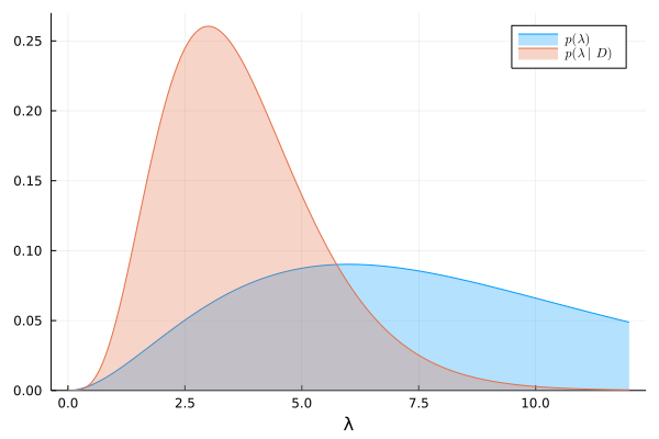
We can visualize the prior and exact posterior:

λ = range(0, 12, length=500)
plot(λ, prior, lab=L"p(\lambda)")
plot!(λ, exact_posterior, lab=L"p(\lambda|D)")

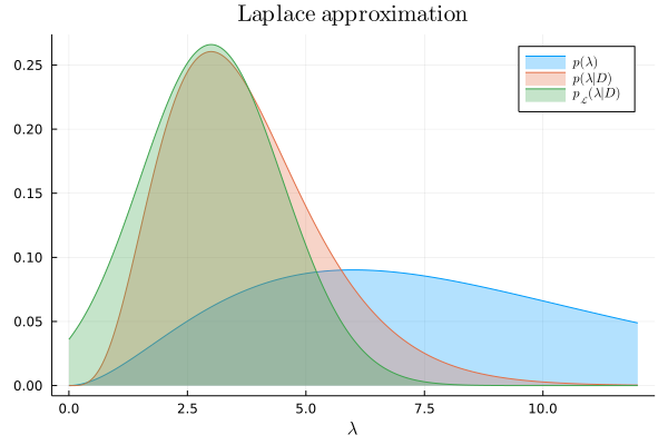
Let's now find the Laplace approximation of the exact posterior using the results we derived. The first step is to find the mode $\lambda_0$ of the joint log-likelihood $\ln p(Y, \lambda)$ . We can do so using the maximize function from the package Optim.jl. The arguments expected by maximize are the function to be maximized and the endpoints of the interval along which the optimization will be performed. The returned object is a structure with several information from which we can extract the mode using the maximizer function.

λ₀ = maximize(joint_log_likelihood(y), first(λ), last(λ)) |> maximizer

The final step is to find $\ln h''(\lambda_0)$ , i.e., the second derivative of the joint log-likelihood $\ln p(Y, \lambda)$ at its mode $\lambda_0$ . We use the derivative function from the ForwardDiff.jl package:

hꜛꜛ(λ) = derivative(λ -> derivative(joint_log_likelihood(y), λ), λ)

Finally, we bring together the pieces to define the Laplace approximation:

laplace_approx = Normal(λ₀, -(hꜛꜛ(λ₀))^(-1))

We can now compare the Laplace approximation to the exact posterior:

plot!(λ, laplace_approx, lab=L"p_{\mathcal{L}}(\lambda|D)", title=L"\textrm{Laplace~approximation}")

A few remarks to conclude this post. The Laplace approximation replaces the problem of integration with that of optimization. This is important because intractable integrals are common in practical applications. On the other hand, even when the integral can be solved, optimization is often faster to compute. However, the Laplace approximation has several limitations: if the posterior distribution being approximated is not unimodal, or does not have it's mass concentrated around the mode, or is not twice-differentiable, then the result will be inaccurate. This is worrying because in many applications we don't have access to the exact posterior, which means that we don't have a reference to test the accuracy of the approximation. In any case, the Laplace approximation has been proven to be effective not only in the context of Bayesian inference, but also in many other mathematical domains that exhibit hard-to-compute integrals.

Credit to @OswaldoGressani for his awesome YouTube video