
This is a gentle introduction to Julia's machine learning toolbox MLJ focused on users new to Julia. In it we train a decision tree to predict whether a new passenger would survive a hypothetical replay of the Titanic disaster. The blog is loosely based on these notebooks.
Prerequisites: No prior experience with Julia, but you should know how to open a Julia REPL session in some terminal or console. A nodding acquaintance with supervised machine learning would be helpful.
Experienced data scientists may want to check out the more advanced tutorial, MLJ for Data Scientists in Two Hours.
Decision Trees
Generally, decision trees are not the best performing machine learning models. However, they are extremely fast to train, easy to interpret, and have flexible data requirements. They are also the building blocks of more advanced models, such as random forests and gradient boosted trees, one of the most successful and widely applied class of machine learning models today. All these models are available in the MLJ toolbox and are trained in the same way as the decision tree.
Here's a diagram representing what a decision tree, trained on the Titanic dataset, might look like:
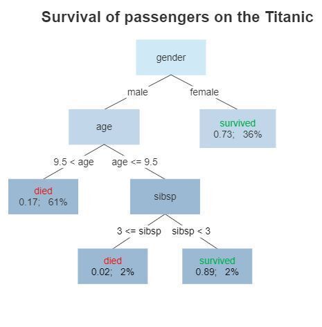
For example, in this model, a male over the age of 9.5 is predicted to die, having a survival probability of 0.17.
Package installation
We start by creating a new Julia package environment called titanic, for tracking versions of the packages we will need. Do this by typing these commands at the julia> prompt, with carriage returns added at the end of each line:
using Pkg
Pkg.activate("titanic", shared=true)
To add the packages we need to your environment, enter the ] character at the julia> prompt, to change it to (titanic) pkg>. Then enter:
add MLJ DataFrames BetaML
It may take a few minutes for these packages to be installed and "precompiled".
Tip. Next time you want to use exactly the same combination of packages in a new Julia session, you can skip the add command and instead just enter the two lines above them.
When the (titanic) pkg> prompt returns, enter status to see the package versions that were installed. Here's what each package does:
MLJ (machine learning toolbox): provides a common interface for interacting with models provided by different packages, and for automating common model-generic tasks, such as hyperparameter optimization demonstrated at the end of this blog.
DataFrames: Allows you to manipulate tabular data that fits into memory. Tip. Checkout these cheatsheets.
BetaML: Provides the core decision algorithm we will be building for Titanic prediction.
Learn more about Julia package management here.
For now, return to the julia> prompt by pressing the "delete" or "backspace" key.
Establishing correct data representation
using MLJ
import DataFrames as DF
After entering the first line above we are ready to use any function in MLJ's documentation as it appears there. After the second, we can use functions from DataFrames, but must qualify the function names with a prefix DF., as we'll see later.
In MLJ, and some other statistics packages, a "scientific type" or scitype indicates how MLJ will interpret data (as opposed to how it is represented on your machine). For example, while we have
julia> typeof(1)
Int64

julia> typeof(true)
Bool
we have
julia> scitype(1)
Count
but also
julia> scitype(true)
Count
Tip. To learn more about a Julia command, use the ? character. For example, try typing ?scitype at the julia> prompt.
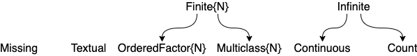
In MLJ, model data requirements are articulated using scitypes, which allows you to focus on what your data represents in the real world, instead of how it is stored on your computer.
Here are the most common "scalar" scitypes:
We'll grab our Titanic data set from OpenML, a platform for sharing machine learning datasets and workflows. The second line below converts the downloaded data into a dataframe.
table = OpenML.load(42638)
df = DF.DataFrame(table)
We can use DataFrames to get summary statistics for the features in our dataset:
DF.describe(df)
| Row | variable | mean | min | median | max | nmissing | eltype |
|---|---|---|---|---|---|---|---|
| 1 | pclass | 1 | 3 | 0 | CategoricalValue{String, UInt32} | ||
| 2 | sex | female | male | 0 | CategoricalValue{String, UInt32} | ||
| 3 | age | 29.7589 | 0.42 | 30.0 | 80.0 | 0 | Float64 |
| 4 | sibsp | 0.523008 | 0.0 | 0.0 | 8.0 | 0 | Float64 |
| 5 | fare | 32.2042 | 0.0 | 14.4542 | 512.329 | 0 | Float64 |
| 6 | cabin | E31 | C148 | 687 | Union{Missing, CategoricalValue{… | ||
| 7 | embarked | C | S | 2 | Union{Missing, CategoricalValue{… | ||
| 8 | survived | 0 | 1 | 0 | CategoricalValue{String, UInt32} |
In particular, we see that cabin has a lot of missing values, and we'll shortly drop it for simplicity.
To get a summary of feature scitypes, we use schema:
schema(df)
| Row | names | scitypes | types |
|---|---|---|---|
| 1 | pclass | Multiclass{3} | CategoricalValue{String, UInt32} |
| 2 | sex | Multiclass{2} | CategoricalValue{String, UInt32} |
| 3 | age | Continuous | Float64 |
| 4 | sibsp | Continuous | Float64 |
| 5 | fare | Continuous | Float64 |
| 6 | cabin | Union{Missing, Multiclass{186}} | Union{Missing, CategoricalValue{… |
| 7 | embarked | Union{Missing, Multiclass{3}} | Union{Missing, CategoricalValue{… |
| 8 | survived | Multiclass{2} | CategoricalValue{String, UInt32} |
Now sibsp represents the number of siblings/spouses, which is not a continuous variable. So we fix that like this:
coerce!(df, :sibsp => Count)
Call schema(df) again, to check a successful change.
Splitting into train and test sets
To objectively evaluate the performance of our final model, we split off 30% of our data into a holdout set, called df_test, which will not used for training:
df, df_test = partition(df, 0.7, rng=123)
You can check the number of observations in each set with DF.nrow(df) and DF.nrow(df_test).
Splitting data into input features and target
In supervised learning, the target is the variable we want to predict, in this case survived. The other features will be inputs to our predictor. The following code puts the df column with name survived into the vector y (the target) and everything else, except cabin, which we're dropping, into a new dataframe called X (the input features).
y, X = unpack(df, ==(:survived), !=(:cabin));
You can check X and y have the expected form by doing schema(X) and scitype(y).
We'll want to do the same for the holdout test set:
y_test, X_test = unpack(df_test, ==(:survived), !=(:cabin));
Choosing a supervised model:
There are not many models that can directly handle missing values and a mixture of scitypes, as we have here. Here's how to list the ones that do:
julia> models(matching(X, y))
 (name = ConstantClassifier, package_name = MLJModels, ... )
 (name = DecisionTreeClassifier, package_name = BetaML, ... )
 (name = DeterministicConstantClassifier, package_name = MLJModels, ... )
 (name = RandomForestClassifier, package_name = BetaML, ... )
This shortcoming can be addressed with data preprocessing provided by MLJ but not covered here, such as one-hot encoding and missing value imputation. We'll settle for the indicated decision tree.
The code for the decision tree model is not available until we explicitly load it, but we can already inspect its documentation. Do this by entering doc("DecisionTreeClassifier", pkg="BetaML"). (To browse all MLJ model documentation use the Model Browser.)
An MLJ-specific method for loading the model code (and necessary packages) is shown below:
Tree = @load DecisionTreeClassifier pkg=BetaML
tree = Tree()
The first line loads the model type, which we've called Tree; the second creates an object storing default hyperparameters for a Tree model. This tree will be displayed thus:
DecisionTreeClassifier(
  max_depth = 0,
  min_gain = 0.0,
  min_records = 2,
  max_features = 0,
  splitting_criterion = BetaML.Utils.gini,
  rng = Random._GLOBAL_RNG())
We can specify different hyperparameters like this:
tree = Tree(max_depth=10)
Training the model
We now bind the data to be used for training and the hyperparameter object tree we just created in a new object called a machine:
mach = machine(tree, X, y)
We train the model on all bound data by calling fit! on the machine. The exclamation mark ! in fit! tells us that fit! mutates (changes) its argument. In this case the model's learned parameters (the actual decision tree) is stored in the mach object:
fit!(mach)
Before getting predictions for new inputs, let's start by looking at predictions for the inputs we trained on:
p = predict(mach, X)
Notice that these are probabilistic predictions. For example, we have
julia> p[6]
           UnivariateFinite{Multiclass{2}}
     ┌                                        ┐
   0 ┤■■■■■■■■■■■■■■■■■■■■■■■■■■■■■■ 0.914894
   1 ┤■■■ 0.0851064
     └                                        ┘
Extracting a raw probability requires an extra step. For example, to get the survival probability (1 corresponding to survival and 0 to death), we do this:
julia> pdf(p[6], "1")
0.0851063829787234
We can also get "point" predictions using the mode function and Julia's broadcasting syntax:
julia> yhat = mode.(p)
julia> yhat[3:5]
3-element CategoricalArrays.CategoricalArray{String,1,UInt32}:
 "0"
 "0"
 "1"
Evaluating model performance
Let's see how accurate our model is at predicting on the data it trained on:
julia> accuracy(yhat, y)
0.921474358974359
Over 90% accuracy! Better check the accuracy on the test data that the model hasn't seen:
julia> yhat = mode.(predict(mach, X_test));
julia> accuracy(yhat, y_test)
0.7790262172284644
Oh dear. We are most likely overfitting the model. Still, not a bad first step.
The evaluation we have just performed is known as holdout evaluation. MLJ provides tools for automating such evaluations, as well as more sophisticated ones, such as cross-validation. See this simple example and the detailed documentation for more information.
Tuning the model
Changing any hyperparameter of our model will alter it's performance. In particular, changing certain parameters may mitigate overfitting.
In MLJ we can "wrap" the model to make it automatically optimize a given hyperparameter, which it does by internally creating its own holdout set for evaluation (or using some other resampling scheme, such as cross-validation) and systematically searching over a specified range of one or more hyperparameters. Let's do that now for our decision tree.
First, we define a hyperparameter range over which to search:
r = range(tree, :max_depth, lower=0, upper=8)
Note that, according to the document string for the decision tree (which we can retrieve now with ?Tree) we see that 0 here means "no limit on max_depth".
Next, we apply MLJ's TunedModel wrapper to our tree, specifying the range and performance measure to use as a basis for optimization, as well as the resampling strategy we want to use, and the search method (grid in this case).
tuned_tree = TunedModel(
    tree,
    tuning = Grid(),
    range=r,
    measure = accuracy,
    resampling=Holdout(fraction_train=0.7),
)
The new model tuned_tree behaves like the old, except that the max_depth hyperparameter effectively becomes a learned parameter instead.
Training this tuned_tree actually performs two operations, under the hood:
Search for the best model using an internally constructed holdout set
Retrain the "best" model on all available data
mach2 = machine(tuned_tree, X, y)
fit!(mach2)
Here's how we can see what the optimal model actually is:
julia> fitted_params(mach2).best_model
DecisionTreeClassifier(
  max_depth = 6,
  min_gain = 0.0,
  min_records = 2,
  max_features = 0,
  splitting_criterion = BetaML.Utils.gini,
  rng = Random._GLOBAL_RNG())
Finally, let's test the self-tuning model on our existing holdout set:
yhat2 = mode.(predict(mach2, X_test))
accuracy(yhat2, y_test)
0.8164794007490637
Although we cannot assign this outcome statistical signicance, without a more detailed analysis, this appears to be an improvement on our original depth=10 model.
Learning more
Suggestions for learning more about Julia and MLJ are here.

Oldest comments (4)
Thanks a lot! Excellent tutorial!
Great tutorial!
This was a really cool post about using Julia for machine learning tasks, especially with the Titanic dataset example. I appreciate the detailed steps on setting up the environment and package management using MLJ and DataFrames. It made things a lot clearer for a beginner like me.
Interestingly, while working with Julia and handling the scitype of variables, I ran into a permission problem on Linux when setting up certain user groups. This guide on how to add user to group Linux really came to my rescue and saved a lot of time.
I love how you included useful tips for managing packages and gave insights on data handling—this is invaluable for learning better machine learning practices. Thanks for sharing!