I try to analyze the daily price of Gold (GLD) with the relationship to the Daily Treasury Par Real Yield Curve Rates using the MLJ regression in Julia.
The Yield Curve Rates has 5-year rate, 7-year rate, 10-year rate, 20-year rate, and 30-year rate. I use all these rates, with its previous from 1 to 4 days values as the features to predict the price of Gold in the next day. Data from 2010–02–22 was collected, and split into training (70%) and testing data (30%). Here is the code in Julia/MLJ I used for the training and testing.
using MLJ
y, X = MLJ.unpack(full_df, ==(Symbol("target")), colname -> true)
train, test = partition(eachindex(y), 0.7)
using MLJLinearModels
reg = @load RidgeRegressor pkg = "MLJLinearModels"
model_reg = reg()
mach = machine(model_reg, X, y)
fit!(mach, rows=train)
yhat = predict(mach, X[test,:])
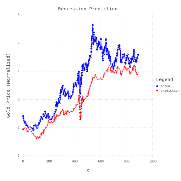
Ridge Regression Model is used for training and prediction. Here is the prediction value compared with the actual value.
Then I tried to use SHAP value to analysis the features importance.
using ShapML
function predict_function(model, data)
  data_pred = DataFrame(y_pred = predict(model, data))
  return data_pred
end
explain = copy(full_df[train, :])
# Remove the outcome column.
explain = select(explain, Not(Symbol("target")))
# An optional reference population to compute the baseline prediction.
reference = copy(full_df)
reference = select(reference, Not(Symbol("target")))
sample_size = 60  # Number of Monte Carlo samples.
data_shap = ShapML.shap(explain = explain,
                         reference = reference,
                         model = mach,
                         predict_function = predict_function,
                         sample_size = sample_size,
                         seed = 1
                         )

show(data_shap, allcols = true)
Then, plot the Mean Absolute Shapley Value with the Gadfly.jl
using Gadfly
data_plot = combine(DataFrames.groupby(data_shap, [:feature_name]),:shap_effect=>mean)
transform!(data_plot,:shap_effect_mean => x -> abs.(x))
data_plot = sort(data_plot, order(:shap_effect_mean_function, rev = true))

baseline = round(data_shap.intercept[1], digits = 1)

p = plot(data_plot, y = :feature_name, x = :shap_effect_mean_function, Coord.cartesian(yflip = true), Scale.y_discrete, Geom.bar(position = :dodge, orientation = :horizontal),Theme(bar_spacing = 1mm),Guide.xlabel("|Shapley effect| (baseline = $baseline)"), Guide.ylabel(nothing),Guide.title("Feature Importance - Mean Absolute Shapley Value"))
draw(PNG("features.png", 6inch, 6inch), p)
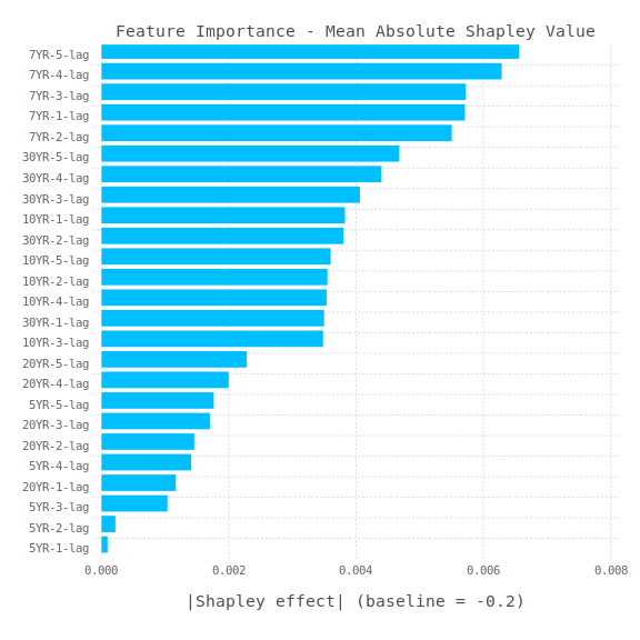
It can be seen that the 7-year yield rate is the most important features. Therefore, the Gold price is related to the 7-year yield rate. However, as the prediction is not fully matched with the actual value, there are other factors affecting the Gold price.
The above is originally posted on my blog in medium.com.

Latest comments (6)
I hate medium, But in love with forem.
Thanks! it was great!
If you go to the settings, you can set the "Canonical URL" to point to your original blog post (this will help with SEO). Also, I manually edited it for you but if you add the word "Julia" after the three back ticks for code, you will get syntax highlighting.
Great work on this!
Nice post. Nice that you show the train-test split. Regarding the Shapley, it's probably better to look at the coefficients directly than estimate them via Shapley values.
forem.julialang.org/rikhuijzer/ran...
That's a model without coefficients
Not sure my understanding is correct, maybe you can shed some light. In a linear model, a higher coefficient for a feature, the more a feature played a role in making a prediction. However, when variables in a regression model are correlated, these conclusions don't hold anymore.