Abstract
- The graphs (curves) output by Plots.jl are polygonal lines, so they look a bit like sharp edges.
- If we use the BasicBSpline.jl package to plot the curve, they will be approximated by Bézier curves, and we'll be happy!
The package used in this article can be installed from Julia's REPL with the following command:
]add Plots
add StaticArrays
add BasicBSpline
add https://github.com/hyrodium/BasicBSplineExporter.jl
Smooth case
Plotting with Plots.jl
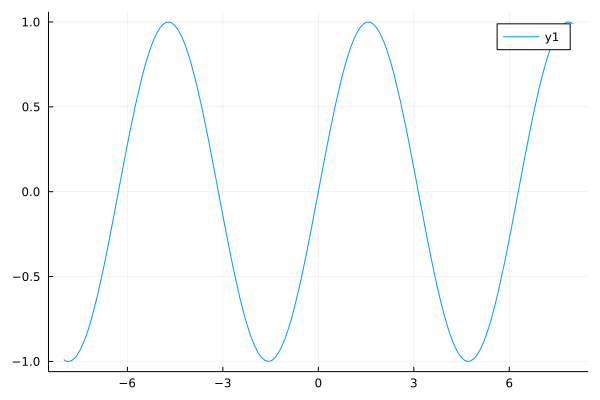
Let's begin by plotting with the Plots.jl package!
using Plots
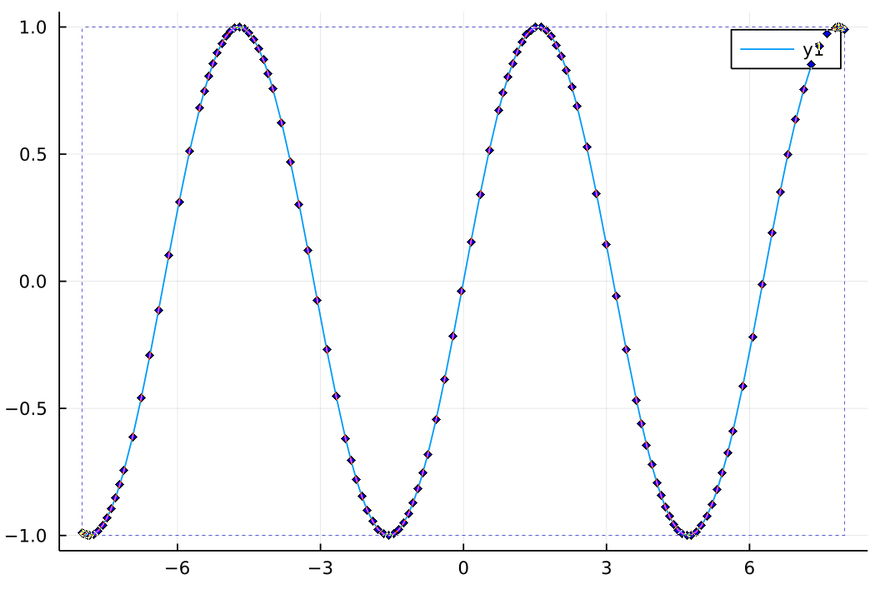
plot(sin,-8,8) # plot sin curve from -8 to 8
savefig("sin_Plots.svg") # save with SVG format
savefig("sin_Plots.png") # save with PNG format
Zoom in on the SVG image near the maxima.
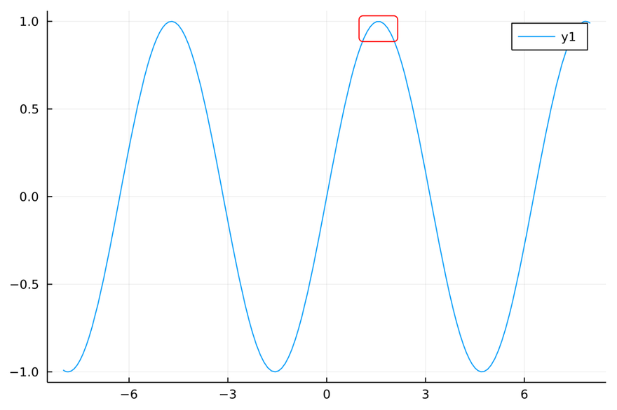
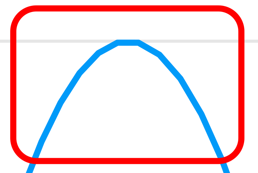
It seems non-smooth curve with sharp edges.
This is because the curve is approximated by a polyline. The following image shows an SVG image opened in Inkscape.
How can we get a smooth graph?
SVG supports Bézier curves, so it should be possible as the file format...
→ Use the BasicBSpline.jl package!
Plotting with BasicBSplineExporter.jl
using BasicBSpline
using BasicBSplineExporter
using StaticArrays

f(t) = SVector(t,sin(t)) # pamametrized sine curve
t0,t1 = -8,8             # endpoints

p = 3                                     # Polynomial degree; SVG allows Bézier curves up to 3rd degree.
k = KnotVector(t0:t1)+p*KnotVector(t0,t1) # Knot vector
P = BSplineSpace{p}(k)                    # B-spline space (piecewise polynomial space)

a = fittingcontrolpoints(f,(P,))  # Calculate control points of B-spline curve
M = BSplineManifold(a,(P,)) # Define B-spline curve
save_svg("sin_BasicBSpline.svg", M, xlims=(-10,10), ylims=(-2,2)) # Save in SVG format
save_png("sin_BasicBSpline.png", M, xlims=(-10,10), ylims=(-2,2)) # Save in PNG format
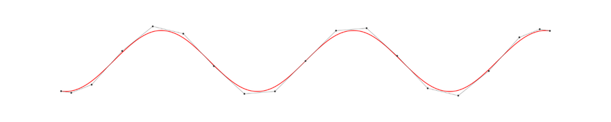
Checking with Inkscape, you can see that the curve is smoothly represented by the Bézier curve as shown below.
The B-spline curve defined above is connected at the knots so that the entire curve is class smooth. Since the curve is polynomial in each section, the curve is represented as a piecewise polynomial.
Non-smooth case
Plotting with Plots.jl
Let's plot a graph of
with Plots.jl
plot(abs∘sin,-8,8)
savefig("abssin_Plots.svg")
savefig("abssin_Plots.png")
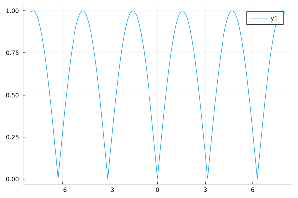
Since this is a polyline approximation, the graph appears to capture the characteristics even at discontinuities in the derivatives.
Plotting with BasicBSplineExporter.jl
As before, graphs can be output by doing the following.
f(t) = SVector(t,abs(sin(t)))
t0,t1 = -8,8
p = 3
k = KnotVector(range(t0,t1,length=50))+p*KnotVector(t0,t1)
P = BSplineSpace{p}(k)
a = fittingcontrolpoints(f,(P,))
M = BSplineManifold(a,(P,))
save_svg("abssin_BasicBSpline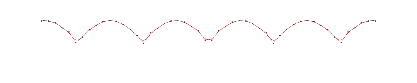.svg", M, xlims=(-10,10), ylims=(-2,2))
save_png("abssin_BasicBSpline.png", M, xlims=(-10,10), ylims=(-2,2))
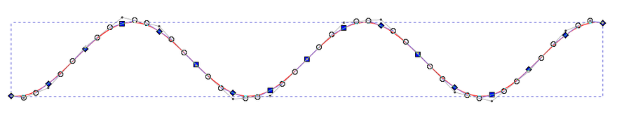
The exported graph↓
Zoom in on the singularity↓
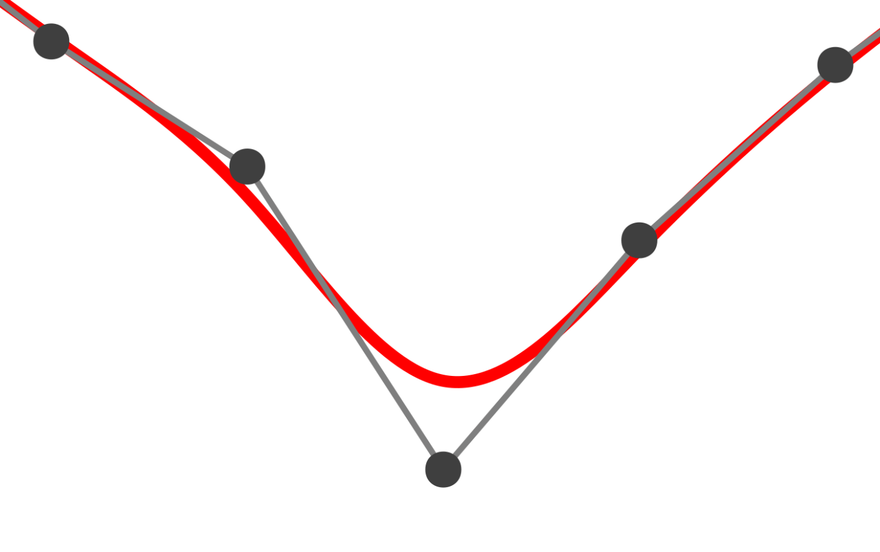
Even if the number of knots (the number of segmented polynomial divisions) is increased, the approximation accuracy will not improve much because of the "smoothly connected" constraint.
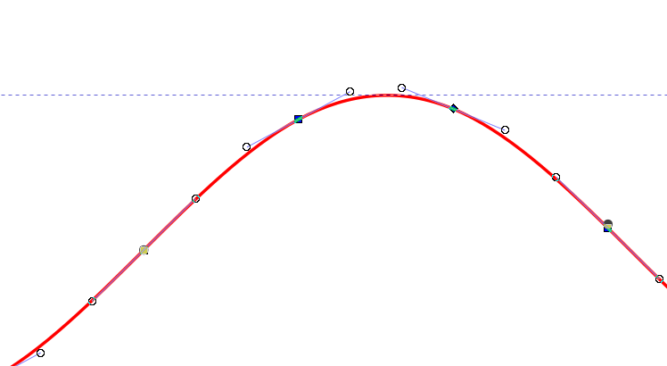
In B-spline theory, it is necessary to place more than one knot at the root of sin because the smoothness of the curve decreases as the knots overlap.
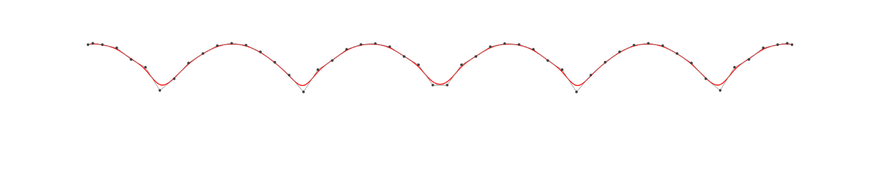
k = KnotVector(range(t0,t1,length=12))+p*KnotVector(t0,t1)
k += p*KnotVector(-2π:π:2π)  # Duplicate knots at points where we want to reduce smoothness
P = BSplineSpace{p}(k)

a = fittingcontrolpoints(f,(P,))
M = BSplineManifold(a,(P,))
save_svg("abssin_BasicBSpline_modified.svg", M, xlims=(-10,10), ylims=(-2,2))
save_png("abssin_BasicBSpline_modified.png", M, xlims=(-10,10), ylims=(-2,2))
The exported graph↓
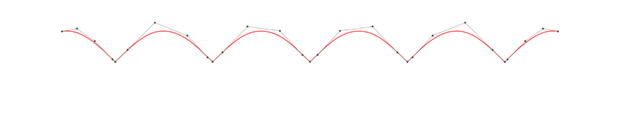
Beautiful even when zoomed in!

Conclusion
- With BasicBSpline.jl package, it's convenient to output smooth graphs!
- B-spline allows you to change the smoothness depending on the overlap of knot vector!
- Plots.jl is a really great package for plotting!
Note: this post is a English translation of this article in zenn.dev.

Top comments (0)