In this post I will give a short introduction on how to automate data acquisition in your experiments using Julia. I will show how PyCall, Makie and JLD2 can be used for these tasks.
Table Of Contents
- Why?
- VISA installation
- PyVISA in Julia
- PyLabLib in Julia
- A tiny experiment
- Saving data and metadata
- Conclusions
Why?
The solution to the two-language problem is something we can take more or less seriously, and try to use Julia for everything humanly possible, or use C or Python with Julia as an intermediary and forget it exists. However, the programmer's need and reasonable judgment must be present to use the right tools for the right tasks. Just as we don't use tweezers to eat a piece of beef, we don't use C++ to write an email from scratch.1
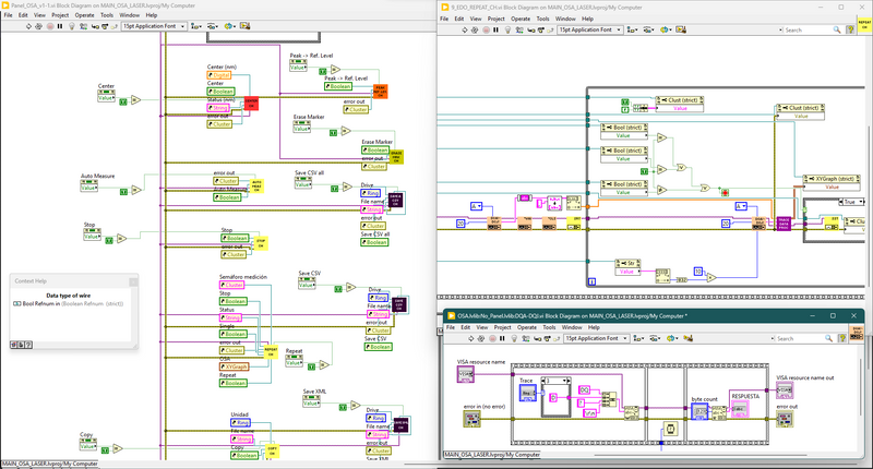
In particular, "the" industry standard for data acquisition system automation and control and test hardware standard is LabVIEW. A software that allows the creation of user interfaces and communication between devices at a very complex level, using a graphical programming paradigm. However, I must point out that: being a proprietary software, we do not know what it does underneath, the licensing terms make it necessary to pay ridiculous amounts of money for tasks that may be simple. And although in principle it is presented as a simple programming paradigm, the code can easily turn into spaghetti, and not figuratively.
Example of a LabVIEW code. This code is intended to control a tunable laser and an Optical Spectrum Analyzer together. As seen, there are many cables, so track the information flux is not always easy.2
Some additional problems I encountered when programming experiment automation in LabVIEW were:
- The lack of version control.
- The software tends to get slow as data arrays get larger, more instruments are connected, or three-dimensional data is plotted for monitoring.
- An absurdly heavy installation.
- A large number of bugs and crashes that are not documented or whose solutions and causes are not clear, even to advanced users in the community forums.
- Broken connections when using the "self-cleaning" tool or simply by saving the .vi file.
- While each function can be programmed in a box, they have such small connections that it is not always easy to connect them. It doesn't help that the software has no close-ups.3
- The program can quickly turn into a ridiculous amount of embedded .vi's, making it easy to have 10 or more windows open during development.
- Poor support for anything other but Windows.
- Arrays! What a pain to declare and use matrices in LabVIEW.
We cannot entirely blame the software, it is a valid solution, so much so that it is a standard. And maybe such insolvencies could be part of a misuse by the user. Personally, however, I don't advocate this position very much.
Instead, it helps that many lab equipment manufacturers liberalize the use of their SDKs and drivers to be used with C, C++, or Python, through (at best) the VISA protocol via SCPI commands and a good base of programming examples, or (at worst) some dll library (whose documentation quality may vary), and typically without Linux support.4
So what does this have to do with Julia? Unfortunately, I have not found a comprehensive discussion of how to use Julia for experiment automation, despite the language's great potential for this purpose:
- Speed, simplicity and clarity.
- Easy handling of matrices and data storage.
- Access to several graphing libraries.
- Access to other programming languages (C, R, Python).
- Compatibility with a version control system (git).
- Synchronous and asynchronous programming access.
- Access to multithreaded and GPU programming.
- Access to programming environments.
This lack of resources means that there is no documentation on how to accomplish these tasks in Julia,5 and essentially no packages exist natively in this language.6
The purpose of this document is therefore to give a small introduction to how to automate experiments in Julia using existing Python solutions such as PyLabLib or PyVISA.7
As a Julia user who does not consider himself to be particularly good at programming, and who does not have too much time to reinvent the wheel,8 or to delve into the world of interfaces and communication protocols, I believe that this small manual can be useful, especially for master's and PhD students who are in a hurry to automate their experiments, but whose main programming language is Julia (yes, we exist).
VISA installation
As a prerequisite, the necessary libraries must be installed. There are two main distributions, National Instruments (NI-VISA), which is the most widely used, and Keysight IO Library Suites. Both support Linux and Windows, but the former is the most widely used and adds macOS X support. Installation instructions are described in the respective links.
There is also PyVISA-py, which covers a subset of the VISA standard functionality, and it appears that it does not support all protocols on all bus systems.9
PyVISA in Julia
As I mentioned before, we will use Python packages in Julia, this because the native packages of Julia (VISA.jl and Instruments.jl) seem to be abandoned. We will install PyCall to access Python, for this we will enter a terminal with Julia to the package manager with the "[" key and execute:
Pkg> add PyCall
We return to the programming environment by pressing the backspace key when the installation is complete. We will now install PyVISA using the following commands:10
using PyCall
run(`$(PyCall.python) -m pip install -U pyvisa`)
If we want to use pyvisa-py in addition, we can install this library thought this command:
run(`$(PyCall.python) -m pip install -U pyvisa-py`)
Let's open a VISA session and list the available devices
# py-visa import
visa = pyimport("pyvisa")

# Now, we open a resource manager. If we give "@py" as argument, we would indicate that we want to use pyvisa-py as the VISA interface.
rm = visa.ResourceManager()

# We list the resources
list_resources = rm_list_resoruces()
This last lane of code will have some output like the following:
julia> list_resources = RM.list_resources()
("USB0::0x0957::0x1798::MYXXXXXXXX::INSTR", "TCPIP0::OSA-MIUP3TTVFTZ::inst0::INSTR", "TCPIP0::192.168.1.120::inst0::INSTR", "TCPIP0::192.168.1.122::inst0::INSTR", "ASRL1::INSTR", "ASRL7::INSTR", "ASRL18::INSTR", "USB0::0x1313::0x8072::1911409::0::INSTR", "USB0::0x1313::0x8078::P0011224::0::INSTR")
These elements are the identification strings of each device connected or visible to the computer. Here we see two devices available on the network via TCPIP and one USB device. We will connect to the USB device and ask it who it is.
# We open a VISA session for this device
OSC = rm.open_resource("USB0::0x0957::0x1798::MYXXXXXXXX::INSTR")
We have three functions at our disposal, write to write instructions to the buffer, read to read the values and responses stored in the buffer, and query, which writes an instruction and then reads the response from the computer (steps 3 and 4). There are more details about this last command that we will see later. Let's ask him who he is:
julia> OSC.query("*IDN?")
"AGILENT TECHNOLOGIES,DSO-X 2014A,MYXXXXXXXX,02.65.2021030741\n"
Note that the string in the argument contains the *IDN? command. This is one of the mandatory commands of the SCIPI standard, and any device that supports VISA must be able to respond to it by returning an identification string. In our case, we see that the device responded with its manufacturer name, model, serial number, and firmware version. The response may vary depending on the manufacturer and the device, but it must provide the necessary information to identify the device; the details of the response string must be included in the user (or programmer) manual.
Let's proceed to acquire and plot the data. To do this, let's define the following function to reset the acquisition parameters and apply an autoscale.
function OSC_inic()
    OSC.write("*RST")
    sleep(1)
    OSC.write(":AUTOSCALE")
    sleep(0.1)
    OSC.write("TIMebase:Scale 2.0E-3")
    sleep(0.1)
    OSC.write("CHANNEL2:DISPLAY 1")
    sleep(0.1)
    OSC.write("CHANNEL2:SCALE 100 mV")
    sleep(0.1)
    OSC.write("CHANNEL1:OFFSet 0 V")
    sleep(0.1)
    OSC.write("CHANNEL1:OFFSet 370 mV")
    sleep(0.1)
end
When we run the function, we get the next behavior11
As a note, the addition of timeouts in the code (using the sleep function) is to allow time for the device to respond. Sometimes instructions may not be written or executed correctly if these timeouts are omitted. The amount of time we need to pause between one instruction and another depends on the device we are using. Sometimes adding such timeouts is unnecessary.
Now that we have the oscilloscope configured, we will proceed to collect the measured data on the screen. To do this, we need to know that the basic operation we will be performing is a query. We know that the device will return a series of numbers, but these may differ in format, as they can be a series of ASCII values or, failing that, binary values. Let's see what happens when we do a simple query
OSC.write("WAVeform:SOURce CHAN1")
OSC.query("WAVeform:DATA?")
And what we get back is a string with the values of the measurement, albeit with an interpretation error. In order for these values to be returned correctly in an array, the following function must be used:
julia> OSC.query_ascii_values("WAVeform:preamble?")
10-element Vector{Float64}:
     0.0
     0.0
 62500.0
     1.0
     3.2e-7
    -0.01
     0.0
     0.4020101
     0.37
   128.0
However, these values are misinterpreted because the oscilloscope output is configured for binary values. Since we know which numbering format our oscilloscope uses, we will use the next function
julia> OSC.query_binary_values("WAVeform:DATA?", datatype="B", is_big_endian=true)
62500-element Vector{Int64}:
 127
 126
 127
 127
 127
   ⋮
 127
 126
 126
 127
 127
This translates the binary value type into a list of numbers, which is more useful for us. But even this is not enough, the values returned by the oscilloscope need to be scaled according to the acquisition configuration of the oscilloscope, so let's define that the returned data is scaled accordingly.
function data_to_values(data, params)
    format, typo, num_points, count, x_incr, x_orig, x_ref, y_incr, y_orig, y_ref = params
    a = 1:puntos
    xs = @. ((a - x_ref) * x_incr) + x_orig
    ys = @. ((data - y_ref) * y_incr) + y_orig
    return [xs, ys]
end
Now, we define a function that automatically returns the data for a specific channel of the oscilloscope.
function OSC_Channel_adq(channel::Int)
    OSC.write("WAVEFORM:SOURCE CHAN$channel")
    sleep(0.1)
    params = OSC.query_ascii_values("wav:preamble?")
    sleep(0.1)
    data = OSC.query_binary_values("WAVeform:DATA?", datatype="B", is_big_endian=true)
    sleep(0.1)
    data_to_values(data, params)
end
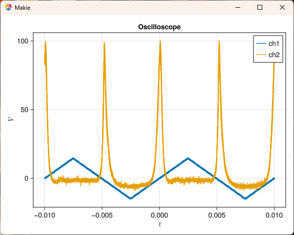
Now, we will use the above to get the data and plot it with GLMakie.jl.
dat_chan_1 = OSC_channel_adq(1)
dat_chan_2 = OSC_channel_adq(2)

using GLMakie
using LaTeXStrings

begin
   f = Figure()
   ax = Axis(f[1,1],
             xlabel = L"t",
             ylabel = L"V",
             title = "Oscilloscope")
   lines!(ax,dat_chan_1...,label="ch. 1")
   lines!(ax,dat_chan_2[1],dat_chan_2[2],label="ch. 2")
   axislegend(ax)
   f
end
To end the VISA session with the oscilloscope, we need to do it correctly with the following command
julia> OSC.close()
It should be noted that each piece of equipment is different, so we must refer to the manual to know how to obtain useful data from the measuring instruments we use.
PyLabLib in Julia
There are devices to which we cannot connect through a VISA session, but we have to do it through their respective controllers. For this we will use PyLabLib, a library that has solved communication with devices of different manufacturers and categories, such as cameras, motors and detectors. The list of supported devices can be found in the package documentation. We will install the full version of the library in PyCall with the following command.
using PyCall
run(`$(PyCall.python) -m pip install -U pylablib"[devio-full]"`)
Let's move on to controlling a Thorlabs K10CR1 rotary mount, for which we must first install the drivers from the following Thorlab's page.
Now, we import the functions that will allow us to control the motor and list the motors connected. We note that the second identified motor is the one we are going to move. We will connect it to inform us which scale it will use according to its model.
julia> Thor = pyimport("pylablib.devices.Thorlabs");

julia> list_thor_devices = Thor.list_kinesis_devices()
2-element Vector{Tuple{String, String}}:
 ("27252406", "Brushed Motor Controller")
 ("55257014", "Kinesis K10CR1 Rotary Stage")

julia> KDC_entr = Thor.KinesisMotor(list_thor_devices[2][1],scale="K10CR1")
Let's see what other functions are available
# List of available functions that can be accessed by pressing the Tab key.
julia> KDC_entr.
CommData                       CommShort                      Error                          NoParameterCaller              __bool__                       __class__
__delattr__                    __dict__                       __dir__                        __doc__                        __enter__                      __eq__
__exit__                       __format__                     __ge__                         __getattribute__               __gt__                         __hash__
__init__                       __init_subclass__              __le__                         __lt__                         __module__                     __ne__
__new__                        __reduce__                     __reduce_ex__                  __repr__                       __setattr__                    __sizeof__
__str__                        __subclasshook__               __weakref__                    _add_device_variable           _add_info_variable             _add_parameter_class
_add_settings_variable         _add_status_variable           _as_parameter_class            _autodetect_stage              _axes                          _axis_parameter_name
_axis_value_case               _bg_msg_counters               _calculate_scale               _call_without_parameters       _close_on_error                _connection_parameters
_cycle_rts                     _d2p                           _default_axis                  _default_get_status            _device_SN                     _device_var_ignore_error
_device_vars                   _device_vars_order             _enable_channel                _find_bays                     _forward_positive              _get_adc_inputs
_get_connection_parameters     _get_device_model              _get_device_variables          _get_gen_move_parameters       _get_homing_parameters         _get_jog_parameters
_get_kcube_trigio_parameters   _get_kcube_trigpos_parameters  _get_limit_switch_parameters   _get_polctl_parameters         _get_position                  _get_scale
_get_stage                     _get_status                    _get_status_n                  _get_step_scale                _get_velocity_parameters       _home
_is_channel_enabled            _is_homed                      _is_homing                     _is_moving                     _is_rack_system                _jog
_make_channel                  _make_dest                     _mapped_axes                   _model                         _model_match                   _move_by
_move_by_mode                  _move_to                       _moving_status                 _multiplex_func                _original_axis_parameter       _p2d
_p_channel_id                  _p_direction                   _p_home_direction              _p_hw_limit_kind               _p_jog_mode                    _p_kcube_trigio_mode
_p_limit_switch                _p_pzmot_channel_enabled       _p_stop_mode                   _p_sw_limit_kind               _parameters                    _pzmot_autoenable
_pzmot_enable_channels         _pzmot_get_drive_parameters    _pzmot_get_enabled_channels    _pzmot_get_jog_parameters      _pzmot_get_kind                _pzmot_get_position
_pzmot_get_status              _pzmot_get_status_n            _pzmot_jog                     _pzmot_kind                    _pzmot_move_by                 _pzmot_move_to
_pzmot_req                     _pzmot_set                     _pzmot_set_position_reference  _pzmot_setup_drive             _pzmot_setup_jog               _pzmot_stop
_pzmot_wait_for_status         _remove_device_variable        _replace_parameter_class       _resolve_axis                  _scale                         _scale_units
_set_position_reference        _set_supported_channels        _setup_comm_parameters         _setup_gen_move                _setup_homing                  _setup_jog
_setup_kcube_trigio            _setup_kcube_trigpos           _setup_limit_switch            _setup_parameter_classes       _setup_polctl                  _setup_velocity
_stage                         _status_comm                   _stop                          _update_axes                   _update_device_variable_order  _wait_for_home
_wait_for_status               _wait_for_stop                 _wait_move                     _wap                           _wip                           _wop
add_background_comm            apply_settings                 blink                          check_background_comm          close                          dv
flush_comm                     get_all_axes                   get_all_channels               get_device_info                get_device_variable            get_full_info
get_full_status                get_gen_move_parameters        get_homing_parameters          get_jog_parameters             get_kcube_trigio_parameters    get_kcube_trigpos_parameters
get_limit_switch_parameters    get_number_of_channels         get_polctl_parameters          get_position                   get_scale                      get_scale_units
get_settings                   get_stage                      get_status                     get_status_n                   get_velocity_parameters        home
instr                          is_homed                       is_homing                      is_moving                      is_opened                      jog
list_devices                   lock                           locking                        move_by                        move_to                        open
query                          recv_comm                      remap_axes                     send_comm                      send_comm_data                 set_default_channel
set_device_variable            set_position_reference         set_supported_channels         setup_gen_move                 setup_homing                   setup_jog
setup_kcube_trigio             setup_kcube_trigpos            setup_limit_switch             setup_polctl                   setup_velocity                 status_bits
stop                           unlock                         using_channel                  wait_for_home                  wait_for_status                wait_for_stop
wait_move
If we are in doubt about what a function does, we can always use Julia's help environment.
help?> KDC_entr.home

        Home the device.

        If ``sync==True``, wait until homing is done (with the given timeout).
        If ``force==False``, only home if the device isn't homed already.
We will do the following, we will send the mount to the home position, and we will define a function that will rotate it to the desired position and inform us of its current position.
const θc_cal = 0.0

function θ_c(θ₀)
    θ = θ₀ - θc_cal
    @info "Moving cube to $(θ₀)°                    "
    KDC_entr.move_to(θ)
    while KDC_entr.get_status()[1] == "moving_bk"
        sleep(0.1)
        print("Cube position,  θ = $(round(KDC_entr.get_position(),digits=4) - θc_cal)°                     \r")
    end
    @info "Cube angle $(θ₀)°                               "
end
Remember to use KDC_1.close() to close the connection when it is no longer needed.
The details of connection, data acquisition, and status checking will vary from device to device. Even the connection to the controllers is different, so I highly recommend consulting the package and instrument documentation to see how these tasks are performed.
Sometimes we have to find the controllers manually, for example the following lines will allow us to connect to the SDK controllers of a monochromator and an Andor camera.
py"""
import pylablib as pll
pll.par["devices/dlls/andor_shamrock"] = "C:\Program Files\Andor SOLIS\Drivers\Shamrock64"
"""
andor = pyimport("pylablib.devices.Andor")
A tiny experiment
Let's take what we've seen so far and measure an optical signal transmitted by a particular device by rotating a polarizer cube, and store the data in the appropriate matrices.
# This code was tested with Julia 1.10.0
using PyCall
using GLMakie
using LaTeXStrings
using ProgressMeter
using JLD2

# Connection with the oscilloscope
visa = pyimport("pyvisa")
RM = visa.ResourceManager()
list_resources = RM.list_resources()
OSC = RM.open_resource(list_resources[1])

@info OSC.query("*IDN?")

# Connection with the motor stage
Thor = pyimport("pylablib.devices.Thorlabs")
list_thor_devices = Thor.list_kinesis_devices()

KDC_entr = Thor.KinesisMotor(list_thor_devices[2][1],scale="K10CR1")

# Definition of oscilloscope's functions
function data_to_values(data, params)
    formato, tipo, puntos, cuenta, x_incr, x_orig, x_ref, y_incr, y_orig, y_ref = params
    a = 1:puntos
    xs = @. ((a - x_ref) * x_incr) + x_orig
    ys = @. ((data - y_ref) * y_incr) + y_orig
    return xs, ys
end

function OSC_Channel_adq(channel::Int)
    OSC.write("WAVEFORM:SOURCE CHAN$channel")
    sleep(0.1)
    params = OSC.query_ascii_values("wav:preamble?")
    sleep(0.1)
    data = OSC.query_binary_values("WAVeform:DATA?", datatype="B", is_big_endian=true)
    sleep(0.1)
    data_to_values(data, params)
end

# Definition of motor stage's functions
θc_cal = 0.0 # Calibration constant
function θ_c(θ₀)
    θ = θ₀ - θc_cal
    @info "Moving cube to $(θ₀)°                    "
    KDC_entr.move_to(θ)
    while KDC_entr.get_status()[1] == "moving_bk"
        sleep(0.1)
        print("Cube at position,  θ = $(round(KDC_entr.get_position(),digits=4) - θc_cal)°                     \r")
    end
    @info "Cube angle $(θ₀)°                               "
end

# Setting matrices sizes
θs = 0:0.5:360
ts1, ch1 = OSC_Channel_adq(1)

ts_ch1 = []
ts_ch2 = []
Data_ch1 = zeros(length(ch1),length(θs))
Data_ch2 = zeros(length(ch1),length(θs))

@showprogress for (i,θ) in enumerate(θs)
   θ_c(θ)
   sleep(0.2)
   t1, V1 = OSC_Channel_adq(1)
   t2, V2 = OSC_Channel_adq(2)
   Data_ch1[:,i] .= V1
   Data_ch2[:,i] .= V2
   push!(ts_ch1,t1)
   push!(ts_ch2,t2)
end

maxs = [maximum(cols) for cols in eachcol(Data_ch1)]
mins = [minimum(cols) for cols in eachcol(Data_ch2)]

extrema_amp = maxs .- mins
Let's plot the amplitudes of the resulting signals.
begin
    F = Figure()
    ax = Axis(F[1,1],
    xlabel=L"\theta \:[^\circ]",
    ylabel=L"V")

    lines!(ax,θs,extrema_amp)
    DataInspector()
    F
end
Experimental data of the transmitted power of a polarized laser through a Glam Taylor polarizer at several degrees.
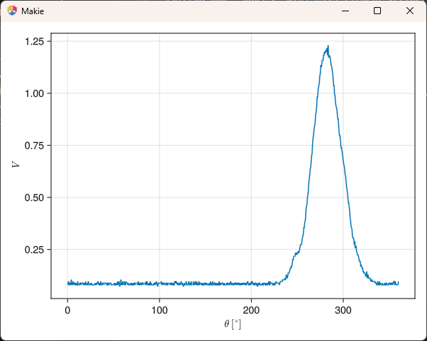
As we can see, the result shows a transmission peak at a certain angle.
Saving data and metadata
In an experiment, it is not enough to save the results of the measurements, we also need to know the conditions under which we made them. In our example above, we need to know what equipment we used, how it was configured, what positions the motor took, or when we ran the experiment.
To store both data and metadata in the same file, we can use the JLD2 package, which allows us to create files compatible with the HDF5 standard. The following sample code defines and executes a function that creates a file containing the configuration parameters of the experiment and the data we measured.
# Save data
file_name = "22012024_malus_1.jld2"
f = jldopen(joinpath("data", file_name), "a+") do file
    configuration = JLD2.Group(file, "configuration")
    datas = JLD2.Group(file, "datas")
    configuration["OSC_preamble"] = OSC.query_ascii_values("wav:preamble?")
    configuration["OSC_idn"] = OSC.query("*IDN?")
    configuration["OSC_conf"] = KDC_entr.get_settings()
    configuration["MOTOR_idn"] = list_thor_devices[2][2]
    datas["ts_ch1"]=ts_ch1
    datas["ts_ch2"]=ts_ch1
    datas["Data_ch1"]=Data_ch1
    datas["Data_ch1"]=Data_ch1
    datas["θs"] = θs
end
If we want to recover the data, we can do it by opening the file. I always suggest that once we are done recovering the data we need, we close the file before processing the data.
julia> a = jldopen("data/24012024_malus_1.jld2")
JLDFile D:\Documentos\Julia-manual-visa\data\24012024_malus_1.jld2 (read-only)
 ├─📂 configuration
 │  ├─🔢 OSC_preamble
 │  ├─🔢 OSC_idn
 │  ├─🔢 OSC_conf
 │  └─🔢 MOTOR_idn
 └─📂 datos
    ├─🔢 ts_ch1
    ├─🔢 ts_ch2
    ├─🔢 Data_ch1
    └─ ⋯ (2 more entries)

julia> OSC_preamble = a["configuration"]["OSC_preamble"]
10-element Vector{Float64}:
     0.0
     0.0
 62500.0
     1.0
     3.2e-7
    -0.01
     0.0
     0.008040201
     0.612
   128.0

julia> close(a)
Conclusions
In this short tutorial I showed the basics of how to automate experiments using instrument communication via PyVISA and PyLabLib. I also briefly showed how to plot the acquired data. At the same time, I showed how to take advantage of instrument communication to store metadata in the same file using the JLD2 package.
I hope this mini-course will be useful, even though it does not cover the potential of the language to apply asynchronous functions, or to generate user interfaces with Makie, dashboards with Genie, or interactive notebooks with Pluto, options that are fully feasible with Julia. At the same time, the implementation of platforms such as DrWatson together with experiment automation techniques seems to be a natural way to have a record of the evolution of the experiments. As a supplement, I leave this link to one of my repositories with the same example we discussed in this tutorial, but implementing some of the ideas I mentioned in this paragraph.
Have fun experimenting!
All trademarks used in this document, as well as images and logos or any other mentioned entity that may appear are the property of their respective owners, and I or this channel claim no right over them.
Facilities available at ICN-UNAM were used for this publication.
-
Of course, this is possible, but I doubt that many users would want to compile code to send a simple email or the meme of the moment. ↩
-
I wrote this code from scratch, programming every single SCIPI command in a .vi file for our OSA, because some years ago their manufacturer only provided code compatible with other models (and .vi's in Japanese!), nowadays there is a usable set of LabVIEW programs, but then this was my only solution. ↩
-
It seems that they tried to solve this with LabVIEW NGX, but the software was somehow incompatible with the traditional version and so damn slow to install and run that they ended up discontinuing it. Addendum: It appears that this functionality was enabled until not too long ago. ↩
-
Or, in the worst case, some software that is free but does not document its drivers, making communication with the device other than through its software very difficult, if not impossible (I'm looking at you, New Focus). ↩
-
It's not that there aren't people discussing it, but it's not a topic that's rich in conversation. This may be the only example of this that I can give you: ↩
-
Although there is Instruments.jl that provides an interface to VISA, I prefer not to use it because at this point it can be considered abandonware. ↩
-
There are also manufacturer's specific solutions, as those provided by Physike Instrumente (PIpython). ↩
-
I once needed to use a function from the C++ Boost library to access special functions not available in SpecialFunctions, it came out regular. Although I was able to run this function sequentially, doing it in parallel was too unstable, so I ended up rewriting the functions I needed in Julia. ↩
-
As mentioned in their documentation. ↩
-
This code is a modification from this answered question in StackOverflow: How to use in Julia a Python package that is not available in Anaconda and needs to be installed via pip ↩
-
The behavior of the oscilloscope in the video corresponds to different scale values with respect to those shown in the code, but otherwise each of the instructions is executed. ↩

Top comments (0)
Some comments may only be visible to logged-in visitors. Sign in to view all comments.