Last week I had to teach for my Computational Linguistics' class the Zipf's Law using Julia. This post includes the Julia code used for demonstrating the Zipf's Law.
I will not spend time on explaining here why this empirically-motivated law that characterizes natural languages holds. I will confine myself here to saying that some brilliant people before the American linguist George Kingsley Zipf spreads the word about its existence noticed a very interesting pattern:
- There are few words in a text that appear most of the times while all the rest appear very few times resulting in a distribution that is reminiscent of the power law distribution.
The goal of this post, however, is to simply demonstrate the validity of the law by using the dataset of the Amazon Musical Instruments Reviews, available in Kaggle.
On the path of achieving this I will be using Julia for handling strings; more specifically, I intend to show how to:
- read in text as a
String - delete punctuation marks and tokenize a string into word tokens
- create a Dictionary with word frequencies
- sort the Dictionary based on word frequencies
- barplotting the frequency values to see the power law-like distribution
Let's take these steps one-by-one.
Reading in text as a String
I will be using the CSV and DataFrames packages to read in the Musical_instruments_reviews.csv file as a DataFrame that contains the Amazon Musical Instruments Reviews.
julia> using DatFrames, CSV

julia> instruments = CSV.read("/Users/atantos/Documents/julia/DataFrames/Instrument_reviews_dataframe/Musical_instruments_reviews.csv", DataFrame);
If you navigate through the instruments DataFrame, you will see that the reviewText column contains the review texts. Each member of the String reviewText column vector is a text. The join() function joins these texts into a single big String that we can further manipulate.
julia> reviewtext = join(instruments.reviewText, " ");
Data Cleaning and Tokenization
The second step is to do some cleaning on the textual data by deleting the punctuation marks and then tokenizing the cleaner output. The following line does the two processing tasks in one step. replace() takes in the reviewed texts and replaces four punctuation marks expressed by the regular expression pattern r"(;|,|\.|!)" with the null string. In other words, it deletes them.
The cleaned text is further tokenized with split using as a splitting criterion the space character " ".
julia> reviewtext_tokens = split(replace(reviewtext,  r"(;|,|\.|!)" => ""), " ")
940593-element Vector{SubString{String}}:
 "Not"
 "much"
 "to"
 "write"
 ⋮
 "recommended"
 "product45/5"
 "stars"
Creating a Word-Frequency Dictionary
The most well-known related counting method in Julia is based on the StatsBase.countmap() function that outputs a Dictionary with words and their frequencies. The first step is to call StasBase's functionality in the current namespace and then we may use its exported function countmap() without needing the package qualification; meaning that we don't need to use the package_name.method() notation, as in StatsBase.countmap(). What countmap() does is that it takes a vector of any type of values and returns a dictionary with keys being the vector elements (the words in our case) and values being the occurrence frequency of these words; namely the elements of the initial vector reviewtext_tokens. Below, word_dict is a dictionary with keys being the vector elements of its argument, reviewtext_tokens and values on the right of the right-pointing arrow are their occurrence frequencies.
julia> using StatsBase

julia> word_dict = countmap(reviewtext_tokens)
Dict{SubString{String}, Int64} with 43812 entries:
  "B0002E2EOE)"           => 1
  "itPS"                  => 1
  "tunerYes"              => 1
  "optionLEVY'S"          => 1
  "whiz"                  => 2
  "simultaneouslyTotally" => 1
  "gathered"              => 2
  ⋮                       => ⋮
Recall that according to Zipf's Law, a few words are very common in a text or corpus of texts and the rest, very rarely, occur. To be able to visualize this asymmetry on the word frequency distribution, we need to first sort the words based on their frequency in decreasing order. Sorting a dictionary based on its values is easy in Julia. The sort() function allows you to use an anonymous function, x->x[2], defined within the named argument by so that you can focus on the values of the Dictionaries' pairs. Notice that for sorting in decreasing order you need to set the rev argument to true.
julia> sorted_word_dict = sort(collect(word_dict), by=x->x[2], rev=true)
43812-element Vector{Pair{SubString{String}, Int64}}:
          "the" => 39206
            "a" => 27175
          "and" => 26223
            "I" => 25333
                ⋮
      "things)" => 1
  "Tone-master" => 1
 "onesMaterial" => 1
Creating a sorted dictionary causes a small complication that one needs to be aware of. Sorted dictionaries have distinct keys and values that are not identical to their unsorted counterparts from which they were constructed. Their keys are the indices of the sorted pair element and their values consist of the key-value pairs of the initial dictionary. This means that in order to access the values of the initial unsorted dictionary that live within the new sorted dictionary, you need to first get the values of the sorted dictionary and ask for the second member of its pairs for retrieving the values with getindex(value, 2). Let's see in practice what I mean by that. Here is the array of keys of the sorted dictionary that contains all the ranking indices .
julia> [key for key in keys(sorted_word_dict)]
43812-element Vector{Int64}:
     1
     2
     3
     4
     ⋮
 43810
 43811
 43812
The values of sorted_word_dict, on the other hand, has the key-value pairs of the initial dictionary word_dict, as you can see:
julia> [value for value in values(sorted_word_dict)]
43812-element Vector{Pair{SubString{String}, Int64}}:
          "the" => 39206
            "a" => 27175
          "and" => 26223
            "I" => 25333
                ⋮
      "things)" => 1
  "Tone-master" => 1
 "onesMaterial" => 1
Keeping the internal structure of sorted_word_dict in mind, below, we are asking for the value of the key-value pairs that live within sorted_word_dict.
julia> freqs=[getindex(value, 2) for value in values(sorted_word_dict)]
43812-element Vector{Int64}:
 39206
 27175
 26223
 25333
     ⋮
     1
     1
     1
To be able to access the keys you need to access the first member of the pairs of the initial unsorted dicitionary that is stored within sorted_word_dict by using getindex(value, 1).
julia> words = [getindex(value, 1) for value in values(sorted_word_dict)]
43812-element Vector{SubString{String}}:
 "the"
 "a"
 "and"
 "I"
 ⋮
 "things)"
 "Tone-master"
 "onesMaterial"
Barplotting with Gadfly
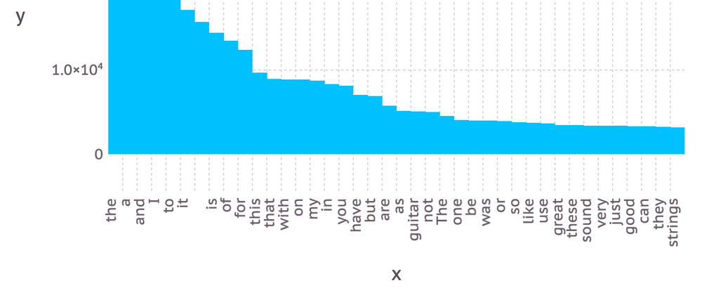
One of the most well-known Julia plotting packages is GadFly. Being a fan of R and its powerful ggplot package, navigating through GadFly's was a breeze.¹ Here is how you could barplot the sorted frequencies of the 40 most frequent words keeping the words as labels on the x-axis and using the dodge position.
julia> using Gadfly

julia> Gadfly.plot(x=words[1:40], y=freqs[1:40], Geom.bar(position=:dodge))
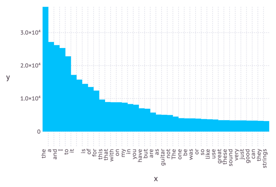
As you can see, the shape of the distribution proves empirically the truth of Zipf's Law.
[1]: Roland Schaetzle wrote an excellent post on TDS that is highly recommended by the Julia community for those who migrate from R to Julia and want to have a similar plotting experience to ggplot.

Latest comments (0)