
Explaining how the algorithm works and the concepts involved is quite difficult and so I shall do it slowly and section by section. I shall refer to the reader as Alice as in the famous character in the Novel "Alice through the Looking Glass". The reason for this is because I need to take the reader into the Looking Glass Universe where things are view differently
Assumptions
In this article I assume that You know
- How to add a package to Julia
- What an XY graph is
- What a Matrix is
- The basic idea of what an inverse of a Matrix is
- The basic idea of what a transpose of a Matrix is
- Basic maths. Addition Subtration. Multiplication. Division. Power.
In this article, I will show you how to perform Least Square Fitting to obtain the parameters of a non-linear model on experimental data.
Step 0 Talk abut the model
In this article we shall model the experimental data using the non-linear model
Y = A exp(B * X) + C
where X,Y are the measurement values from the experiment and
A,B,C are the unknown constants.
The unknown constants are also refer to as the parameters
We generalise this by saying
Y = f(x) and
f(x) = A exp(B * x) + C
Now this function f is very important and it represent the relationship between X and Y. That is to say: Given X, what is Y?
Later on in the article we will use the function f to get a "Looking Glass" function g by stepping through the Looking Glass. Naturally the function g is highly related to the function f . We shall talk about this later.
Step 1 Obtaining experimental data
We could perform the experiment and obtain lots of values of X and Y but for this article we shall generate the values using a deterministic random number generator.
Here is the source code for generating the values of X and Y
using Distributions, StableRNGs

#=
We want to generate Float64 data deterministically
=#

function generatedata(formula; input=[Float64(_) for _ in 0:(8-1)], seed=1234, digits=0,
    preamble="rawdata = ", noisedist=Normal(0.0, 0.0), verbose=true)
    vprint(verbose, str) = print(verbose == true ? str : "")
    local myrng = StableRNG(seed)
    local array = formula.(input) + rand(myrng, noisedist, length(input))
    if digits > 0
        array = round.(array, digits=digits)
    end
    vprint(verbose, preamble)
    # Now print the begining array symbol '['
    vprint(verbose, "[")
    local counter = 0
    local firstitem = true
    for element in array
        if firstitem == true
            firstitem = false
        else
            vprint(verbose, ",")
        end
        counter += 1
        if counter % 5 == 1
            vprint(verbose, "\n  ")
        end
        vprint(verbose, element)
    end
    vprint(verbose, "]\n")
    return array
end

A_actual = 1.5
B_actual = -0.25
C_actual = 3.5
f(x) = A_actual * exp(B_actual * x) + C_actual
numofsamples = 400+1
X = [Float64(_) for _ in 0:0.01:(numofsamples-1)/100]
Y = generatedata(f, input=X, digits=5, noisedist=Normal(0.0, 0.0005), preamble="Y = ",verbose=false)
println("\n\nX = ", X, "\nY = ", round.(Y,digits=5), "\n\n")
with the output
X = [0.0, 0.01, 0.02, 0.03, 0.04, 0.05, 0.06, 0.07, 0.08, 0.09, 0.1, 0.11, 0.12, 0.13, 0.14, 0.15, 0.16, 0.17, 0.18, 0.19, 0.2, 0.21, 0.22, 0.23, 0.24, 0.25, 0.26, 0.27, 0.28, 0.29, 0.3, 0.31, 0.32, 0.33, 0.34, 0.35, 0.36, 0.37, 0.38, 0.39, 0.4, 0.41, 0.42, 0.43, 0.44, 0.45, 0.46, 0.47, 0.48, 0.49, 0.5, 0.51, 0.52, 0.53, 0.54, 0.55, 0.56, 0.57, 0.58, 0.59, 0.6, 0.61, 0.62, 0.63, 0.64, 0.65, 0.66, 0.67, 0.68, 0.69, 0.7, 0.71, 0.72, 0.73, 0.74, 0.75, 0.76, 0.77, 0.78, 0.79, 0.8, 0.81, 0.82, 0.83, 0.84, 0.85, 0.86, 0.87, 0.88, 0.89, 0.9, 0.91, 0.92, 0.93, 0.94, 0.95, 0.96, 0.97, 0.98, 0.99, 1.0, 1.01, 1.02, 1.03, 1.04, 1.05, 1.06, 1.07, 1.08, 1.09, 1.1, 1.11, 1.12, 1.13, 1.14, 1.15, 1.16, 1.17, 1.18, 1.19, 1.2, 1.21, 1.22, 1.23, 1.24, 1.25, 1.26, 1.27, 1.28, 1.29, 1.3, 1.31, 1.32, 1.33, 1.34, 1.35, 1.36, 1.37, 1.38, 1.39, 1.4, 1.41, 1.42, 1.43, 1.44, 1.45, 1.46, 1.47, 1.48, 1.49, 1.5, 1.51, 1.52, 1.53, 1.54, 1.55, 1.56, 1.57, 1.58, 1.59, 1.6, 1.61, 1.62, 1.63, 1.64, 1.65, 1.66, 1.67, 1.68, 1.69, 1.7, 1.71, 1.72, 1.73, 1.74, 1.75, 1.76, 1.77, 1.78, 1.79, 1.8, 1.81, 1.82, 1.83, 1.84, 1.85, 1.86, 1.87, 1.88, 1.89, 1.9, 1.91, 1.92, 1.93, 1.94, 1.95, 1.96, 1.97, 1.98, 1.99, 2.0, 2.01, 2.02, 2.03, 2.04, 2.05, 2.06, 2.07, 2.08, 2.09, 2.1, 2.11, 2.12, 2.13, 2.14, 2.15, 2.16, 2.17, 2.18, 2.19, 2.2, 2.21, 2.22, 2.23, 2.24, 2.25, 2.26, 2.27, 2.28, 2.29, 2.3, 2.31, 2.32, 2.33, 2.34, 2.35, 2.36, 2.37, 2.38, 2.39, 2.4, 2.41, 2.42, 2.43, 2.44, 2.45, 2.46, 2.47, 2.48, 2.49, 2.5, 2.51, 2.52, 2.53, 2.54, 2.55, 2.56, 2.57, 2.58, 2.59, 2.6, 2.61, 2.62, 2.63, 2.64, 2.65, 2.66, 2.67, 2.68, 2.69, 2.7, 2.71, 2.72, 2.73, 2.74, 2.75, 2.76, 2.77, 2.78, 2.79, 2.8, 2.81, 2.82, 2.83, 2.84, 2.85, 2.86, 2.87, 2.88, 2.89, 2.9, 2.91, 2.92, 2.93, 2.94, 2.95, 2.96, 2.97, 2.98, 2.99, 3.0, 3.01, 3.02, 3.03, 3.04, 3.05, 3.06, 3.07, 3.08, 3.09, 3.1, 3.11, 3.12, 3.13, 3.14, 3.15, 3.16, 3.17, 3.18, 3.19, 3.2, 3.21, 3.22, 3.23, 3.24, 3.25, 3.26, 3.27, 3.28, 3.29, 3.3, 3.31, 3.32, 3.33, 3.34, 3.35, 3.36, 3.37, 3.38, 3.39, 3.4, 3.41, 3.42, 3.43, 3.44, 3.45, 3.46, 3.47, 3.48, 3.49, 3.5, 3.51, 3.52, 3.53, 3.54, 3.55, 3.56, 3.57, 3.58, 3.59, 3.6, 3.61, 3.62, 3.63, 3.64, 3.65, 3.66, 3.67, 3.68, 3.69, 3.7, 3.71, 3.72, 3.73, 3.74, 3.75, 3.76, 3.77, 3.78, 3.79, 3.8, 3.81, 3.82, 3.83, 3.84, 3.85, 3.86, 3.87, 3.88, 3.89, 3.9, 3.91, 3.92, 3.93, 3.94, 3.95, 3.96, 3.97, 3.98, 3.99, 4.0]
Y = [5.00026, 4.99671, 4.99168, 4.98814, 4.98473, 4.98102, 4.97771, 4.97393, 4.96957, 4.96567, 4.96252, 4.96015, 4.9556, 4.95183, 4.94868, 4.94439, 4.94139, 4.93792, 4.93397, 4.93044, 4.92662, 4.92324, 4.91925, 4.91613, 4.91287, 4.90931, 4.90609, 4.90147, 4.89842, 4.89508, 4.89157, 4.8876, 4.88476, 4.88175, 4.87781, 4.87462, 4.87074, 4.86746, 4.86411, 4.86027, 4.8575, 4.85359, 4.84989, 4.84682, 4.84404, 4.83992, 4.83673, 4.83395, 4.83077, 4.82657, 4.82314, 4.82066, 4.81735, 4.81311, 4.80956, 4.80774, 4.80396, 4.80025, 4.79692, 4.79453, 4.79056, 4.78834, 4.78521, 4.78146, 4.77902, 4.77504, 4.77291, 4.76972, 4.7647, 4.76251, 4.75913, 4.75643, 4.75262, 4.7496, 4.74612, 4.74393, 4.74016, 4.73748, 4.73441, 4.73105, 4.72772, 4.72505, 4.72198, 4.71788, 4.71669, 4.71308, 4.71046, 4.70721, 4.70349, 4.70032, 4.69721, 4.69474, 4.69145, 4.68943, 4.68538, 4.68237, 4.68024, 4.67703, 4.67413, 4.67229, 4.66888, 4.66589, 4.66264, 4.65933, 4.65577, 4.65449, 4.65059, 4.64823, 4.6461, 4.6431, 4.6392, 4.63667, 4.63245, 4.63044, 4.62859, 4.62477, 4.62197, 4.62009, 4.61724, 4.61425, 4.6117, 4.6092, 4.60616, 4.60314, 4.59975, 4.5978, 4.59554, 4.59203, 4.58831, 4.58639, 4.58263, 4.58192, 4.57885, 4.5761, 4.57306, 4.57052, 4.56772, 4.56495, 4.56203, 4.55984, 4.55683, 4.55441, 4.55088, 4.54908, 4.54606, 4.54433, 4.54214, 4.53836, 4.5362, 4.53241, 4.53141, 4.52867, 4.52551, 4.52338, 4.52062, 4.51883, 4.51532, 4.51249, 4.51068, 4.50698, 4.50629, 4.50336, 4.50098, 4.49811, 4.49508, 4.49317, 4.48983, 4.48791, 4.48504, 4.48337, 4.48136, 4.4778, 4.47559, 4.47316, 4.4703, 4.46867, 4.46528, 4.46452, 4.45991, 4.45953, 4.45685, 4.45328, 4.45157, 4.44927, 4.44621, 4.44493, 4.4421, 4.43922, 4.43794, 4.43555, 4.43322, 4.43068, 4.42809, 4.4264, 4.42316, 4.42128, 4.41914, 4.41739, 4.41406, 4.41157, 4.40969, 4.4076, 4.40453, 4.40268, 4.40096, 4.39855, 4.39654, 4.39399, 4.39193, 4.3892, 4.38635, 4.38445, 4.38312, 4.38146, 4.37867, 4.37581, 4.37449, 4.37264, 4.3692, 4.36779, 4.36556, 4.36366, 4.36077, 4.3589, 4.3578, 4.35527, 4.35167, 4.34997, 4.3491, 4.3457, 4.34382, 4.34193, 4.3396, 4.33865, 4.33591, 4.33407, 4.33229, 4.32937, 4.32821, 4.3259, 4.32237, 4.32102, 4.31951, 4.31657, 4.31483, 4.31291, 4.31125, 4.30921, 4.30641, 4.30484, 4.3028, 4.301, 4.29897, 4.29732, 4.29448, 4.29281, 4.28975, 4.28915, 4.2868, 4.2858, 4.28295, 4.28058, 4.28009, 4.27766, 4.27502, 4.27358, 4.27174, 4.2687, 4.26786, 4.26582, 4.26392, 4.26183, 4.25931, 4.25732, 4.25707, 4.25473, 4.25133, 4.24999, 4.24787, 4.24655, 4.24507, 4.24296, 4.24149, 4.23917, 4.23702, 4.2357, 4.23442, 4.23145, 4.23031, 4.22895, 4.22615, 4.22453, 4.22319, 4.22086, 4.21921, 4.21783, 4.21609, 4.21384, 4.21163, 4.21076, 4.20879, 4.2065, 4.20493, 4.20258, 4.20095, 4.19956, 4.19858, 4.19528, 4.19366, 4.19288, 4.1901, 4.18912, 4.1877, 4.18586, 4.18422, 4.18253, 4.18112, 4.17955, 4.17818, 4.17609, 4.17396, 4.17281, 4.17105, 4.16854, 4.16699, 4.16667, 4.16367, 4.16227, 4.16073, 4.15925, 4.15801, 4.15625, 4.15331, 4.15193, 4.15034, 4.14909, 4.14783, 4.14581, 4.14392, 4.14243, 4.1407, 4.13978, 4.13744, 4.13692, 4.13441, 4.13327, 4.13116, 4.13048, 4.12872, 4.12701, 4.1243, 4.12402, 4.12258, 4.11982, 4.11875, 4.11768, 4.11669, 4.1146, 4.11309, 4.11081, 4.10998, 4.10841, 4.10661, 4.10511, 4.10405, 4.10142, 4.10056, 4.09889, 4.09851, 4.09635, 4.09528, 4.09188, 4.09195, 4.0895, 4.08858, 4.08764, 4.0859, 4.08428, 4.08316, 4.08134, 4.07975, 4.07809, 4.07754, 4.07452, 4.0756, 4.07306, 4.07144, 4.06975, 4.06911, 4.06743, 4.06596, 4.06462, 4.06311, 4.06288, 4.05962, 4.05898, 4.05684, 4.05688, 4.05526, 4.05294, 4.05135]
Step 2 Doing the Least Square Fitting on the experimental data
We show you the source code for the algorithmn and the output first and later in the article we shall explain how the algorithmn works.
"""
Provide the solution to the nonlinear Least Square
"""
function nonlinearLSQ(xarray, yarray; maxiter=8, startpos=[ 1.0 , -0.1, 1.0 ], stepsize=1.0, verbose=true)
    len_xarray = length(xarray)
    len_yarray = length(yarray)
    if len_xarray != len_yarray
        println("Error in function nonlinearLSQ: length of xarray != length of yarray")
        return nothing
    end
    # Parameter array P = [ A , B , C ]
    P = startpos  # Initial Starting Position
    for iteration = 1:maxiter
        R = zeros(len_yarray) # a len_yarray size array
        # Let's create the J Matrix (Jacobian Matrix)
        J = zeros(len_yarray, 3) # a len_yarray*3 matrix
        for i = 1:len_yarray
            J[i, 1] = exp(P[2] * X[i])
            J[i, 2] = P[1] * exp(P[2] * X[i]) * X[i]
            J[i, 3] = 1.0
            R[i] = yarray[i] - (  P[1] * exp(P[2] * xarray[i]) + P[3]  )
        end
        # Dont forget to reshape values from
        # a 1D vector R into a len*1 column matrix RR
        local RR = reshape(R, len_yarray, 1) # a len_yarray * 1 Matrix
        DeltaP = inv(J' * J) * J' * RR
        # At this point the varible DeltaP is a len_yarray * 1 Matrix
        # We turn it into an 1 dimensional vector using vec() function
        P = P + stepsize .* vec( DeltaP )
        if verbose == true
            println("Iteration is ",iteration)
            println(" DeltaP is ",round.(DeltaP,digits=5))
            println(" P is ",round.(P,digits=5))
        end
    end
    println()
    return P
end

solution = nonlinearLSQ(X, Y, maxiter=8, startpos=[ 1.0 , -0.1, 1.0 ])
println("Trying with startpos [ 1.0 , -0.1 , 1.0 ] stepsize=1.0 maxiter=8")
println("The estimate for A is ", round.(solution[1],digits=5))
println("The estimate for B is ", round.(solution[2],digits=5))
println("The estimate for C is ", round.(solution[3],digits=5))
With the output
Iteration is 1
 DeltaP is [-1.58274; -0.42322; 4.57972;;]
 P is [-0.58274, -0.52322, 5.57972]
Iteration is 2
 DeltaP is [1.82102; -0.53788; -1.82729;;]
 P is [1.23828, -1.0611, 3.75242]
Iteration is 3
 DeltaP is [-0.34721; 0.78483; 0.28928;;]
 P is [0.89107, -0.27627, 4.0417]
Iteration is 4
 DeltaP is [0.601; 0.04232; -0.53397;;]
 P is [1.49208, -0.23395, 3.50773]
Iteration is 5
 DeltaP is [0.00431; -0.01652; -0.00425;;]
 P is [1.49638, -0.25047, 3.50349]
Iteration is 6
 DeltaP is [0.00429; 0.00069; -0.00425;;]
 P is [1.50067, -0.24979, 3.49923]
Iteration is 7
 DeltaP is [1.0e-5; -0.0; -1.0e-5;;]
 P is [1.50068, -0.24979, 3.49923]
Iteration is 8
 DeltaP is [0.0; 0.0; -0.0;;]
 P is [1.50068, -0.24979, 3.49923]

Trying with startpos [ 1.0 , -0.1 , 1.0 ] stepsize=1.0 maxiter=8
The estimate for A is 1.50068
The estimate for B is -0.24979
The estimate for C is 3.49923
Step 3 Discussing how Jacobian Matrix is constructed in the code.
In the source code, it was mentioned that you need to create the Jacobian Matrix. Now you may want to read the wikipedia article below on how to create the Jacobian Matrix but I found the wikipedia article to be confusing for newbies.
https://en.wikipedia.org/wiki/Jacobian_matrix_and_determinant
The reason the wikipedia article is confusing is that it talks about a function f but that f is referred to a particular generic function related to the issue at hand.
I have modified the content of the wikipedia article to better reflect our problem and it looks like this.
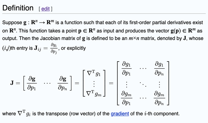
Now time for some explaination. The Matrix p is a 3x1 parameter matrix. It consists of

Now the function g on the otherhand is a family of functions.
Because we have 401 data points from the experiment. Namely
Now Alice, we come back to the function f which we mentioned at the start of the article. As you recall, we had the non-linear model
Y = A exp(B * X) + C
where X,Y are the measurement values from the experiment and
A,B,C are the unknown constants.
Which we generalise by saying
Y = f(x) and
f(x) = A exp(B * x) + C
Now Alice, understand that this is TRUE before we perform the experiment. That is to say X and Y are variables while A, B and C are the unknown constants.
That is to say
X can be any value(s)
Y can be any value(s)
but
A is a fixed value (but currently unknown)
B is a fixed value (but currently unknown)
C is a fixed value (but currently unknown)
And the WHOLE POINT of the experiment is to determine the values of A, B and C
Now it is time to enter the Looking Glass by performing the experiment. Once we had perform the experiment, we are in the MAGICAL REALM of the LOOKING GLASS and things change:
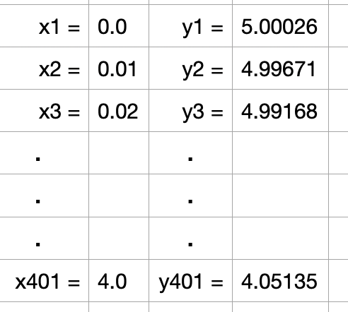
X and Y are now a list of FIXED value pairs
x1 , y1
x2 , y2
.
.
.
x401 , y401
We represent this by saying x and y is a 401x1 column matrix
And we represent it by
y = g(p)
Where g is a family of functions consists of
g is a 1x401 matrix of
g1(A,B,C) = A exp(B * x1) + C
g2(A,B,C) = A exp(B * x2) + C
g3(A,B,C) = A exp(B * x3) + C
.
.
.
g401(A,B,C) = A exp(B * x401) + C
Which in this case, we can say g(A,B,C) is a function related to the function of f(x)
Now when we put in the values of x1 , x2 , x3 , ... , x401 from the experimental results, we get
g1(A,B,C) = A exp(B * 0.0) + C
g2(A,B,C) = A exp(B * 0.01) + C
g3(A,B,C) = A exp(B * 0.02) + C
.
.
.
g401(A,B,C) = A exp(B * 4.0) + C
It is important to know WHAT HAS CHANGED
That is to say X and Y are constants while A, B and C are now variables
That is to say
X is FIXED (by the values obtained from the experiment)
Y is FIXED (by the values obtained from the experiment)
but
A can be any value
B can be any value
C can be any value
We need to do this because we wanted to differentiate the variables A , B and C and we cannot (technically) differentiate a constant.
So back to generating the Jacobian Matrix
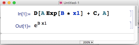
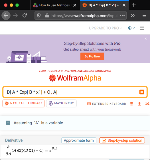
We need to find the partial derivative of g1 in respect to A
in particular
g1(A,B,C) = A exp(B * x1) + C
There are 3 ways
- Using Mathematica
- Using Wolfram Alpha
- Doing it by hand
Using Mathematica
Using Wolfram Alpha
using url https://www.wolframalpha.com
Doing it by hand
Too lazy to do it by hand, Here are the basic steps
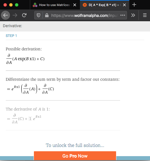
The equivalent part of the source code is
J[i, 1] = exp(P[2] * X[i])
Remember P[2] is the variable B
Partial derivative with respect to B
Next We need to find the partial derivative of g1 in respect to B
in particular
g1(A,B,C) = A exp(B * x1) + C
The answer is A * exp(B * x1) * x1
Which is reflected in the source code
J[i, 2] = P[1] * exp(P[2] * X[i]) * X[i]
Partial derivative with respect to C
Finally We need to find the partial derivative of g1 in respect to C
in particular
g1(A,B,C) = A exp(B * x1) + C
The answer is 1
Which is reflected in the source code
J[i, 3] = 1.0
Step 4 Discussing how the algorithm works. Multiple explainations. Pick one that you like
How does the algorithmn work?
There are many explanation of the algorithm works. Here are some of the explainations
First we calculate
r_i = y_i - g_i(p)
We want g_i(p) to be exactly y_i so
r_i = 0 (since g_i(p) is exactly y_i)
Now this is a function r_i(p) which we can diffentiate using the Jacobian matrix.
Now, what is a Jacobian? A Jacobian is the equivalence of a multidimensional derivative analog of a function expressed in a matrix format. With the importance on the fact that it is multidimensional.
So
Jacobian(r) = Jacobian(y - g(p))
Jacobian(r) = Jacobian(-g(p)) since y is a constant
Jacobian(r) = -1 * Jacobian(g(p))
therefore
p_1 = p_0 - Jacobian(r(p_0))
p_1 = p_0 + Jacobian(g(p_0))
Please note that given p_i the Jacobian(r(p_i)) points to a direction that is the maximum increases of r(p_i) (ie maximum gradient).
in general, if you start with a parameter estimate p_i , you can get a better estimate with.
p_(i+1) = p_i - Jacobian(r(p_i))
thus
p_(i+1) = p_i + Jacobian(g(p_i))
So we can continously update the value of p
Step 5 Discussing the effect of the step size
Our starting pos is
solution = nonlinearLSQ(X, Y, maxiter=8, startpos=[ 1.0 , -0.1, 1.0 ])
And what happens next is
pos[0] is [ 1.0 , -0.1 , 1.0 ]

Our first step is
DeltaP is [-1.58274; -0.42322; 4.57972;;]
pos[1] is [-0.58274, -0.52322, 5.57972]

Our second step is
DeltaP is [1.82102; -0.53788; -1.82729;;]
pos[2] is [1.23828, -1.0611, 3.75242]

Our third step is
DeltaP is [-0.34721; 0.78483; 0.28928;;]
pos[3] is [0.89107, -0.27627, 4.0417]

Our fourth step is
DeltaP is [0.601; 0.04232; -0.53397;;]
pos[4] is [1.49208, -0.23395, 3.50773]

Our fifth step is
DeltaP is [0.00431; -0.01652; -0.00425;;]
pos[5] is [1.49638, -0.25047, 3.50349]

Our sixth step is
DeltaP is [0.00429; 0.00069; -0.00425;;]
pos[6] is [1.50067, -0.24979, 3.49923]

Our seventh step is
DeltaP is [1.0e-5; -0.0; -1.0e-5;;]
pos[7] is [1.50068, -0.24979, 3.49923]

Our eigth step is
DeltaP is [0.0; 0.0; -0.0;;]
pos[8] is [1.50068, -0.24979, 3.49923]
Noticed that our step are gradually getting smaller and smaller.
So why do we start with startpos = [ 1.0 , -0.1 , 1.0 ]? Because I knew the answer is 1.5 , -0.25 , 3.5 . I know the answer is that because I builted up the raw data in the first place.
But what if we do not know what the answer is?
Then I woud have started the program with the startpos of [ 1.0 , -1.0 , 1.0 ] being a generic starting point. I tend to avoid values of 0.0
So what happens when we start with that startpos instead? We get
Trying with startpos [ 1.0 , -1.0 , 1.0 ] stepsize=1.0 maxiter=8

pos[0] is [ 1.0 , -1.0 , 1.0 ]
Iteration is 1
DeltaP is [-0.08045; 0.88542; 3.02142;;]
pos[1] is [0.91955, -0.11458, 4.02142]
Iteration is 2
DeltaP is [-0.71245; -0.37299; 0.76899;;]
pos[2] is [0.20711, -0.48757, 4.79041]
Iteration is 3
DeltaP is [1.06606; 1.33297; -1.0707;;]
pos[3] is [1.27317, 0.8454, 3.71972]
Iteration is 4
DeltaP is [-1.46498; 0.03173; 1.33635;;]
pos[4] is [-0.19181, 0.87712, 5.05607]
Iteration is 5
DeltaP is [0.01914; -0.19153; -0.0255;;]
pos[5] is [-0.17267, 0.68559, 5.03056]
Iteration is 6
DeltaP is [-0.15717; -0.37635; 0.19506;;]
pos[6] is [-0.32984, 0.30924, 5.22562]
Iteration is 7
DeltaP is [-1.23965; -0.65218; 1.30354;;]
pos[7] is [-1.5695, -0.34294, 6.52916]
Iteration is 8
DeltaP is [3.00069; -0.07667; -2.96156;;]
pos[8] is [1.43119, -0.41961, 3.5676]

The estimate for A is 1.43119
The estimate for B is -0.41961
The estimate for C is 3.5676
The important thing is that we get the WRONG answer. But why? The ANSWER is that we keep overstepping the correct answer and we didn't take enough steps. If we tried with MORE steps:
solution = nonlinearLSQ(X, Y, startpos=[ 1.0 , -1.0, 1.0 ],
maxiter=18,
verbose=true)
Trying with startpos [ 1.0 , -1.0 , 1.0 ] stepsize=1.0 maxiter=18
Iteration is 1
 DeltaP is [-0.08045; 0.88542; 3.02142;;]
 P is [0.91955, -0.11458, 4.02142]
Iteration is 2
 DeltaP is [-0.71245; -0.37299; 0.76899;;]
 P is [0.20711, -0.48757, 4.79041]
Iteration is 3
 DeltaP is [1.06606; 1.33297; -1.0707;;]
 P is [1.27317, 0.8454, 3.71972]
Iteration is 4
 DeltaP is [-1.46498; 0.03173; 1.33635;;]
 P is [-0.19181, 0.87712, 5.05607]
Iteration is 5
 DeltaP is [0.01914; -0.19153; -0.0255;;]
 P is [-0.17267, 0.68559, 5.03056]
Iteration is 6
 DeltaP is [-0.15717; -0.37635; 0.19506;;]
 P is [-0.32984, 0.30924, 5.22562]
Iteration is 7
 DeltaP is [-1.23965; -0.65218; 1.30354;;]
 P is [-1.5695, -0.34294, 6.52916]
Iteration is 8
 DeltaP is [3.00069; -0.07667; -2.96156;;]
 P is [1.43119, -0.41961, 3.5676]
Iteration is 9
 DeltaP is [-0.08597; 0.14295; 0.08345;;]
 P is [1.34522, -0.27666, 3.65105]
Iteration is 10
 DeltaP is [0.14663; 0.02842; -0.14309;;]
 P is [1.49185, -0.24823, 3.50796]
Iteration is 11
 DeltaP is [0.00879; -0.00157; -0.00869;;]
 P is [1.50064, -0.2498, 3.49926]
Iteration is 12
 DeltaP is [4.0e-5; 1.0e-5; -4.0e-5;;]
 P is [1.50068, -0.24979, 3.49923]
Iteration is 13
 DeltaP is [-0.0; -0.0; 0.0;;]
 P is [1.50068, -0.24979, 3.49923]
Iteration is 14
 DeltaP is [0.0; 0.0; -0.0;;]
 P is [1.50068, -0.24979, 3.49923]
Iteration is 15
 DeltaP is [0.0; -0.0; 0.0;;]
 P is [1.50068, -0.24979, 3.49923]
Iteration is 16
 DeltaP is [-0.0; -0.0; 0.0;;]
 P is [1.50068, -0.24979, 3.49923]
Iteration is 17
 DeltaP is [0.0; 0.0; -0.0;;]
 P is [1.50068, -0.24979, 3.49923]
Iteration is 18
 DeltaP is [0.0; 0.0; -0.0;;]
 P is [1.50068, -0.24979, 3.49923]

The estimate for A is 1.50068
The estimate for B is -0.24979
The estimate for C is 3.49923
Then we get the right ANSWER
Or we could try with a half step size
solution = nonlinearLSQ(X, Y, startpos=[ 1.0 , -1.0, 1.0 ],
maxiter=(8*2), stepsize=(1.0/2),
verbose=true )
Trying with startpos [ 1.0 , -1.0 , 1.0 ] stepsize=0.5 maxiter=(8*2)
Iteration is 1
 DeltaP is [-0.08045; 0.88542; 3.02142;;]
 P is [0.95978, -0.55729, 2.51071]
Iteration is 2
 DeltaP is [0.24708; 0.36408; 1.2708;;]
 P is [1.08332, -0.37525, 3.14611]
Iteration is 3
 DeltaP is [0.31175; 0.14463; 0.45672;;]
 P is [1.23919, -0.30294, 3.37447]
Iteration is 4
 DeltaP is [0.2326; 0.05843; 0.15327;;]
 P is [1.35549, -0.27372, 3.45111]
Iteration is 5
 DeltaP is [0.13803; 0.02526; 0.05519;;]
 P is [1.42451, -0.26109, 3.47871]
Iteration is 6
 DeltaP is [0.07442; 0.01163; 0.02225;;]
 P is [1.46172, -0.25528, 3.48983]
Iteration is 7
 DeltaP is [0.03853; 0.00557; 0.00982;;]
 P is [1.48098, -0.25249, 3.49474]
Iteration is 8
 DeltaP is [0.01959; 0.00272; 0.00459;;]
 P is [1.49078, -0.25113, 3.49704]
Iteration is 9
 DeltaP is [0.00987; 0.00135; 0.00222;;]
 P is [1.49571, -0.25046, 3.49814]
Iteration is 10
 DeltaP is [0.00496; 0.00067; 0.00109;;]
 P is [1.49819, -0.25012, 3.49869]
Iteration is 11
 DeltaP is [0.00248; 0.00033; 0.00054;;]
 P is [1.49943, -0.24995, 3.49896]
Iteration is 12
 DeltaP is [0.00124; 0.00017; 0.00027;;]
 P is [1.50005, -0.24987, 3.49909]
Iteration is 13
 DeltaP is [0.00062; 8.0e-5; 0.00013;;]
 P is [1.50037, -0.24983, 3.49916]
Iteration is 14
 DeltaP is [0.00031; 4.0e-5; 7.0e-5;;]
 P is [1.50052, -0.24981, 3.49919]
Iteration is 15
 DeltaP is [0.00016; 2.0e-5; 3.0e-5;;]
 P is [1.5006, -0.2498, 3.49921]
Iteration is 16
 DeltaP is [8.0e-5; 1.0e-5; 2.0e-5;;]
 P is [1.50064, -0.24979, 3.49922]

The estimate for A is 1.50064
The estimate for B is -0.24979
The estimate for C is 3.49922
We can even try with one-tenth the step size
#=
  Try it with [ 1.0 , -1.0 , 1.0 ] stepsize=0.1
=#

solution = nonlinearLSQ(X, Y, startpos=[ 1.0 , -1.0, 1.0 ],
    maxiter=(8*10), stepsize=(1.0/10),
    verbose=false)
println("Trying with startpos [ 1.0 , -1.0 , 1.0 ] stepsize=0.1 maxiter=(8*10)")
println("The estimate for A is ", round.(solution[1],digits=5))
println("The estimate for B is ", round.(solution[2],digits=5))
println("The estimate for C is ", round.(solution[3],digits=5))
With the result
Trying with startpos [ 1.0 , -1.0 , 1.0 ] stepsize=0.1 maxiter=(8*10)
The estimate for A is 1.50016
The estimate for B is -0.24992
The estimate for C is 3.49907
Step 6 Further Improvements
One obvious improvement is to compute the two step sizes
- full step
- half step
and then "decide" which step is the appropriate step.
We can do this by comparing the fitness value of each step by applying a fitness function to each candidate step size. We then choose the step with the greatest fitness value (smallest error).
That is to say "fitness value" = 1.0/abs(error)
"""
Provide the solution to the linear Least Square Version 2
"""
function nonlinearLSQ_ver2(xarray, yarray; maxiter=8, startpos=[ 1.0 , -0.1, 1.0 ], verbose=true)
    len_xarray = length(xarray)
    len_yarray = length(yarray)
    if len_xarray != len_yarray
        println("Error in function nonlinearLSQ: length of xarray != length of yarray")
        return nothing
    end
    # Now define our error function
    function abserrorfunc(xarray,yarray,P)
        local i
        local abserrorvalue = 0.0
        for i = 1:length(yarray)
            abserrorvalue += (yarray[i] - (  P[1] * exp(P[2] * xarray[i]) + P[3]  ))^2.0
        end
        return abserrorvalue
    end
    # Now define our fitness function
    function fitness(xarray,yarray,P)
        return 1.0/abserrorfunc(xarray,yarray,P)
    end
    # Parameter array P = [ A , B , C ]
    P = startpos  # Initial Starting Position
    for iteration = 1:maxiter
        R = zeros(len_yarray) # a len_yarrayx1 column matrix
        # Let's create the J Matrix (Jacobian Matrix)
        J = zeros(len_yarray, 3) # a len_yarray*3 matrix
        for i = 1:len_yarray
            J[i, 1] = exp(P[2] * X[i])
            J[i, 2] = P[1] * exp(P[2] * X[i]) * X[i]
            J[i, 3] = 1.0
            R[i] = yarray[i] - (  P[1] * exp(P[2] * xarray[i]) + P[3]  )
        end
        # Dont forget to reshape values from
        # a 1D vector R into a len*1 column matrix RR
        local RR = reshape(R, len_yarray, 1) # a len_yarray * 1 Matrix
        DeltaP = inv(J' * J) * J' * RR
        # Define our two stepsizes
        local fullstep = 1.0 .* vec( DeltaP )
        local halfstep = 0.5 .* vec( DeltaP )
        # Calculate fitness value for both stepsize
        local fitnessvalue_fullstep = fitness(xarray,yarray,P + fullstep)
        local fitnessvalue_halfstep = fitness(xarray,yarray,P + halfstep)
        # Choose the step with the greatest fitness value
        local appropriatestep
        if fitnessvalue_fullstep >= fitnessvalue_halfstep
            appropriatestep = "fullstep"
            P = P + fullstep
        else
            appropriatestep = "halfstep"
            P = P + halfstep
        end
        if verbose == true
            println("Iteration is ",iteration)
            println(" DeltaP is ",round.(DeltaP,digits=5))
            println("The appropriate step size is ",appropriatestep)
            println(" P is ",round.(P,digits=5))
        end
    end
    println()
    return P
end

#=
  Try it with [ 1.0 , -1.0 , 1.0 ]
=#
println("Trying with Version 2 with startpos [ 1.0 , -1.0 , 1.0 ] maxiter=8")
solution = nonlinearLSQ_ver2(X, Y, startpos=[ 1.0 , -1.0, 1.0 ],
    maxiter=18,
    verbose=true)
println("")
println("The estimate for A is ", round.(solution[1],digits=5))
println("The estimate for B is ", round.(solution[2],digits=5))
println("The estimate for C is ", round.(solution[3],digits=5))
print("\n\n")
with output
Trying with Version 2 with startpos [ 1.0 , -1.0 , 1.0 ] maxiter=8
Iteration is 1
 DeltaP is [-0.08045; 0.88542; 3.02142;;]
The appropriate step size is fullstep
 P is [0.91955, -0.11458, 4.02142]
Iteration is 2
 DeltaP is [-0.71245; -0.37299; 0.76899;;]
The appropriate step size is halfstep
 P is [0.56333, -0.30108, 4.40592]
Iteration is 3
 DeltaP is [0.91013; 0.12439; -0.87981;;]
The appropriate step size is fullstep
 P is [1.47345, -0.17669, 3.52611]
Iteration is 4
 DeltaP is [-0.13223; -0.0919; 0.13188;;]
The appropriate step size is fullstep
 P is [1.34122, -0.26859, 3.65799]
Iteration is 5
 DeltaP is [0.15487; 0.02025; -0.15423;;]
The appropriate step size is fullstep
 P is [1.4961, -0.24834, 3.50376]
Iteration is 6
 DeltaP is [0.00455; -0.00146; -0.0045;;]
The appropriate step size is fullstep
 P is [1.50064, -0.2498, 3.49926]
Iteration is 7
 DeltaP is [3.0e-5; 1.0e-5; -3.0e-5;;]
The appropriate step size is fullstep
 P is [1.50068, -0.24979, 3.49923]
Iteration is 8
 DeltaP is [-0.0; -0.0; 0.0;;]
The appropriate step size is fullstep
 P is [1.50068, -0.24979, 3.49923]


The estimate for A is 1.50068
The estimate for B is -0.24979
The estimate for C is 3.49923
If you have 3 or more step sizes then you need version 3 of the code below
"""
Provide the solution to the linear Least Square Version 3
"""
function nonlinearLSQ_ver3(xarray, yarray; maxiter=8, startpos=[ 1.0 , -0.1, 1.0 ], verbose=true)
    len_xarray = length(xarray)
    len_yarray = length(yarray)
    if len_xarray != len_yarray
        println("Error in function nonlinearLSQ: length of xarray != length of yarray")
        return nothing
    end
    # Now define our error function
    function abserrorfunc(xarray,yarray,P)
        local i
        local abserrorvalue = 0.0
        for i = 1:length(yarray)
            abserrorvalue += (yarray[i] - (  P[1] * exp(P[2] * xarray[i]) + P[3]  ))^2.0
        end
        return abserrorvalue
    end
    # Parameter array P = [ A , B , C ]
    P = startpos  # Initial Starting Position
    for iteration = 1:maxiter
        R = zeros(len_yarray) # a len_yarrayx1 column matrix
        # Let's create the J Matrix (Jacobian Matrix)
        J = zeros(len_yarray, 3) # a len_yarray*3 matrix
        for i = 1:len_yarray
            J[i, 1] = exp(P[2] * X[i])
            J[i, 2] = P[1] * exp(P[2] * X[i]) * X[i]
            J[i, 3] = 1.0
            R[i] = yarray[i] - (  P[1] * exp(P[2] * xarray[i]) + P[3]  )
        end
        # Dont forget to reshape values from
        # a 1D vector R into a len*1 column matrix RR
        local RR = reshape(R, len_yarray, 1) # a len_yarray * 1 Matrix
        DeltaP = inv(J' * J) * J' * RR
        # Define our various stepsizes
        local fullstep         = (1.0/1.0)   .* vec( DeltaP )
        local halfstep         = (1.0/2.0)   .* vec( DeltaP )
        local quarterstep      = (1.0/4.0)   .* vec( DeltaP )
        local eighthstep       = (1.0/8.0)   .* vec( DeltaP )
        local sixteenthstep    = (1.0/16.0)  .* vec( DeltaP )
        # Calculate error value for various stepsize
        local errorvalue_fullstep        = abserrorfunc(xarray,yarray,P + fullstep)
        local errorvalue_halfstep        = abserrorfunc(xarray,yarray,P + halfstep)
        local errorvalue_quarterstep     = abserrorfunc(xarray,yarray,P + quarterstep)
        local errorvalue_eighthstep      = abserrorfunc(xarray,yarray,P + eighthstep)
        local errorvalue_sixteenthstep   = abserrorfunc(xarray,yarray,P + sixteenthstep)
        # Create an array of tuples
        local resultarray = Tuple{Float64, Vector{Float64}, String}[]
        push!(resultarray,  (errorvalue_fullstep,fullstep,"fullstep")  )
        push!(resultarray,  (errorvalue_halfstep,halfstep,"halfstep")  )
        push!(resultarray,  (errorvalue_quarterstep,quarterstep,"quarterstep")  )
        push!(resultarray,  (errorvalue_eighthstep,eighthstep,"eighthstep")  )
        push!(resultarray,  (errorvalue_sixteenthstep,sixteenthstep,"sixteenthstep")  )
        # Choose the step with the smallest error value

        local sortedresultarray = sort(resultarray,lt=(A,B)->A[1]<B[1])
        local appropriatestep = sortedresultarray[1][3]
        local correctstep = sortedresultarray[1][2]

        P = P + correctstep

        if verbose == true
            println("Iteration is ",iteration)
            println(" DeltaP is ",round.(DeltaP,digits=5))
            println("The appropriate step size is ",appropriatestep)
            println("The correct step is ",round.(correctstep,digits=5))
            println(" P is ",round.(P,digits=5))
        end
    end
    println()
    return P
end

#=
  Try it with [ 1.0 , -1.0 , 1.0 ]
=#
println("Trying with Version 3 with startpos [ 1.0 , -1.0 , 1.0 ] maxiter=8")
solution = nonlinearLSQ_ver3(X, Y, startpos=[ 1.0 , -1.0, 1.0 ],
    maxiter=8,
    verbose=true)
println("")
println("The estimate for A is ", round.(solution[1],digits=5))
println("The estimate for B is ", round.(solution[2],digits=5))
println("The estimate for C is ", round.(solution[3],digits=5))
print("\n\n")
with the result
Trying with Version 3 with startpos [ 1.0 , -1.0 , 1.0 ] maxiter=8
Iteration is 1
 DeltaP is [-0.08045; 0.88542; 3.02142;;]
The appropriate step size is fullstep
The correct step is [-0.08045, 0.88542, 3.02142]
 P is [0.91955, -0.11458, 4.02142]
Iteration is 2
 DeltaP is [-0.71245; -0.37299; 0.76899;;]
The appropriate step size is quarterstep
The correct step is [-0.17811, -0.09325, 0.19225]
 P is [0.74144, -0.20783, 4.21367]
Iteration is 3
 DeltaP is [0.72118; -0.09448; -0.67662;;]
The appropriate step size is fullstep
The correct step is [0.72118, -0.09448, -0.67662]
 P is [1.46263, -0.30231, 3.53705]
Iteration is 4
 DeltaP is [0.00973; 0.04897; -0.00986;;]
The appropriate step size is fullstep
The correct step is [0.00973, 0.04897, -0.00986]
 P is [1.47236, -0.25334, 3.52719]
Iteration is 5
 DeltaP is [0.02814; 0.0036; -0.02778;;]
The appropriate step size is fullstep
The correct step is [0.02814, 0.0036, -0.02778]
 P is [1.50049, -0.24975, 3.49941]
Iteration is 6
 DeltaP is [0.00018; -4.0e-5; -0.00018;;]
The appropriate step size is fullstep
The correct step is [0.00018, -4.0e-5, -0.00018]
 P is [1.50068, -0.24979, 3.49923]
Iteration is 7
 DeltaP is [0.0; 0.0; -0.0;;]
The appropriate step size is fullstep
The correct step is [0.0, 0.0, -0.0]
 P is [1.50068, -0.24979, 3.49923]
Iteration is 8
 DeltaP is [-0.0; -0.0; 0.0;;]
The appropriate step size is fullstep
The correct step is [-0.0, -0.0, 0.0]
 P is [1.50068, -0.24979, 3.49923]


The estimate for A is 1.50068
The estimate for B is -0.24979
The estimate for C is 3.49923

Top comments (0)